Basis Splines
This chapter describes functions for the computation of smoothing basis splines (B-splines). A smoothing spline differs from an interpolating spline in that the resulting curve is not required to pass through each data point. For information about interpolating splines, see Interpolation.
The header file gsl_bspline.h contains the prototypes for the
bspline functions and related declarations.
Overview
Basis splines are commonly used to fit smooth curves to data sets.
They are defined on some interval ![[a,b]](_images/math/c47bfde07e072efe45e71eb8b5e6891be77ec2df.png) which is sub-divided
into smaller intervals by defining a non-decreasing sequence of knots.
Between any two adjacent knots, a B-spline of order
which is sub-divided
into smaller intervals by defining a non-decreasing sequence of knots.
Between any two adjacent knots, a B-spline of order  is a
polynomial of degree
is a
polynomial of degree  , and so B-splines defined over the
whole interval are called piecewise polynomials. In
order to generate a smooth spline spanning the full interval, the
different polynomial pieces are often required to match one or more
derivatives at the knots.
, and so B-splines defined over the
whole interval are called piecewise polynomials. In
order to generate a smooth spline spanning the full interval, the
different polynomial pieces are often required to match one or more
derivatives at the knots.
B-splines of order are basis functions
for spline functions of the same order, so that all possible spline
functions on some interval can be expressed as linear combinations
of B-splines,

Here, the  coefficients
  are known as
control points and are often determined from a least squares fit.
The
are known as
control points and are often determined from a least squares fit.
The  are the basis splines of order ,
and depend on a knot vector
are the basis splines of order ,
and depend on a knot vector  , which is a non-decreasing
sequence of
, which is a non-decreasing
sequence of  knots
knots

On each knot interval  , the B-splines
  are polynomials of degree .
The basis splines of order are defined by
are polynomials of degree .
The basis splines of order are defined by

for  . The common case of cubic B-splines
is given by
. The common case of cubic B-splines
is given by  . The above recurrence relation can be
evaluated in a numerically stable way by the de Boor algorithm.
. The above recurrence relation can be
evaluated in a numerically stable way by the de Boor algorithm.
In what follows, we will drop the and simply refer
to the spline functions as  and
and  for simplicity,
with the understanding that each set of spline basis functions depends on
the chosen knot vector . We will also occasionally
drop the order and use
for simplicity,
with the understanding that each set of spline basis functions depends on
the chosen knot vector . We will also occasionally
drop the order and use  and
interchangeably.
and
interchangeably.
Vector Splines
The spline above can be generalized to vector control points,

where the  may have some length
  .
.
Knot vector
In practice, one will often identify locations inside the interval
where it makes sense to end one polynomial piece and
begin another. These locations are called interior knots or breakpoints.
It may be desirable to increase the density of knots in regions with rapid
changes, and decrease the density when the underlying data is changing slowly.
For some applications it may be simply best to distribute the knots with
equal spacing on the interval, which are called uniform knots.
The full knot vector will look like

The  interior knots are in . In order to have a full
basis of B-splines, we require an additional
interior knots are in . In order to have a full
basis of B-splines, we require an additional  exterior knots,
 and
and  .
These knots must satisfy
.
These knots must satisfy

but can otherwise be arbitrary.
Allocation of B-splines
-
type gsl_bspline_workspace
The computation of B-spline functions requires a preallocated workspace.
-
gsl_bspline_workspace *gsl_bspline_alloc(const size_t k, const size_t nbreak)
-
gsl_bspline_workspace *gsl_bspline_alloc_ncontrol(const size_t k, const size_t ncontrol)
These functions allocate a workspace for computing B-splines of order
k. The number of breakpoints is given bynbreak. Alternatively, the number of control points may be specified in ncontrol. The relationship is . Cubic B-splines
are specified by . The size of the workspace is
. Cubic B-splines
are specified by . The size of the workspace is
 .
.
-
void gsl_bspline_free(gsl_bspline_workspace *w)
This function frees the memory associated with the workspace
w.
Initializing the knots vector
-
int gsl_bspline_init_augment(const gsl_vector *tau, gsl_bspline_workspace *w)
This function initializes the knot vector
using the
non-decreasing interior knot vector tauof length by
choosing the exterior knots to be equal to the first and last interior knot.
The total knot vector is
by
choosing the exterior knots to be equal to the first and last interior knot.
The total knot vector is
where
 is specified by the
  -th element of
 tau.This function does not verify that the
tauvector is non-decreasing, so the user must ensure this.
-
int gsl_bspline_init_uniform(const double a, const double b, gsl_bspline_workspace *w)
This function constructs a knot vector using uniformly spaced interior knots on
and
sets the exterior knots to the interval endpoints.
The total knot vector is
with

-
int gsl_bspline_init_periodic(const double a, const double b, gsl_bspline_workspace *w)
This function constructs a knot vector suitable for defining a periodic B-spline on
with a period  . There are several ways to choose a periodic knot vector.
Here, we adopt the approach of Dierckx, 1982, and require
. There are several ways to choose a periodic knot vector.
Here, we adopt the approach of Dierckx, 1982, and require
We further define a uniform spacing between each consecutive knot pair. The knot values are given by

-
int gsl_bspline_init_interp(const gsl_vector *x, gsl_bspline_workspace *w)
This function calculates a knot vector suitable for interpolating data at the
abscissa values provided in x, which must be in ascending order. The knot vector for interpolation must satisfy the Schoenberg-Whitney conditions,
This function selects the knots according to

which satisfy the Schoenberg-Whitney conditions, although this may not be the optimal knot vector for a given interpolation problem.
-
int gsl_bspline_init_hermite(const size_t nderiv, const gsl_vector *x, gsl_bspline_workspace *w)
This function calculates a knot vector suitable for performing Hermite interpolation data at the
abscissa values provided in x, which must be in ascending order. The parameternderivspecifies the maximum derivative order which will be interpolated.The knot vector has length
 , where
  , and is given by,
This function uses the convention that
 and
and  . See
Mummy (1989) for more details.
. See
Mummy (1989) for more details.
-
int gsl_bspline_init(const gsl_vector *t, gsl_bspline_workspace *w)
This function sets the knot vector equal to the user-supplied vector
twhich must have length and be non-decreasing.
Properties of B-splines
-
size_t gsl_bspline_ncontrol(const gsl_bspline_workspace *w)
This function returns the number of B-spline control points given by
 .
.
-
size_t gsl_bspline_order(const gsl_bspline_workspace *w)
This function returns the B-spline order
.
-
size_t gsl_bspline_nbreak(const gsl_bspline_workspace *w)
This function returns the number of breakpoints (interior knots) defined for the B-spline.
Evaluation of B-splines
-
int gsl_bspline_calc(const double x, const gsl_vector *c, double *result, gsl_bspline_workspace *w)
This function evaluates the B-spline

at the point
xgiven the control points c. The result is stored in result. Ifxlies outside the knot interval, a Taylor series approximation about the closest knot endpoint is used to extrapolate the spline.
-
int gsl_bspline_vector_calc(const double x, const gsl_matrix *c, gsl_vector *result, gsl_bspline_workspace *w)
This function evaluates the vector valued B-spline

at the point
xgiven the control vectors .
The vector is stored in the -th column of c. The result is stored in
 result. The parameterscandresultmust have the same number of rows. Ifxlies outside the knot interval, a Taylor series approximation about the closest knot endpoint is used to extrapolate the spline.
-
int gsl_bspline_basis(const double x, gsl_vector *B, size_t *istart, gsl_bspline_workspace *w)
This function evaluates all potentially nonzero B-spline basis functions at the position
xand stores them in the vectorBof length, so that the -th element is  for
for
 . The output
 istartis guaranteed to be in![[0, n - k]](_images/math/2b3dc1346098620d135009c9f3e18f613a19009d.png) .
By returning only the nonzero basis functions, this function
allows quantities involving linear combinations of the
to be computed without unnecessary terms
(such linear combinations occur, for example,
when evaluating an interpolated function).
.
By returning only the nonzero basis functions, this function
allows quantities involving linear combinations of the
to be computed without unnecessary terms
(such linear combinations occur, for example,
when evaluating an interpolated function).
Evaluation of B-spline derivatives
-
int gsl_bspline_calc_deriv(const double x, const gsl_vector *c, const size_t nderiv, double *result, gsl_bspline_workspace *w)
This function evaluates the B-spline derivative

at the point
xgiven the control points c. The derivative order is specified by
 nderiv. The result is stored in
 result. Ifxlies outside the knot interval, a Taylor series approximation about the closest knot endpoint is used to extrapolate the spline.
-
int gsl_bspline_vector_calc_deriv(const double x, const gsl_matrix *c, const size_t nderiv, gsl_vector *result, gsl_bspline_workspace *w)
This function evaluates the vector valued B-spline derivative

at the point
xgiven the control vectors .
The vector is stored in the -th column of c. The result is stored in
 result. The parameterscandresultmust have the same number of rows. The derivative order is specified in nderiv. Ifxlies outside the knot interval, a Taylor series approximation about the closest knot endpoint is used to extrapolate the spline.
-
int gsl_bspline_basis_deriv(const double x, const size_t nderiv, gsl_matrix *dB, size_t *istart, gsl_bspline_workspace *w)
This function evaluates all potentially nonzero B-spline basis function derivatives of orders
 through
 nderiv(inclusive) at the positionxand stores them in the matrixdB. The -th element of
 dBis .
The last row of
.
The last row of dBcontains .
The matrix
.
The matrix dBmust be of size by at least  .
The output
.
The output istartis guaranteed to be in.
Note that function evaluations are included as the zeroth order derivatives in dB. By returning only the nonzero basis functions, this function allows quantities involving linear combinations of the and
their derivatives to be computed without unnecessary terms.
Evaluation of B-spline integrals
-
int gsl_bspline_calc_integ(const double a, const double b, const gsl_vector *c, double *result, gsl_bspline_workspace *w)
This function computes the integral

using the coefficients stored in
cand the integration limits (a,b). The integral value is stored inresulton output.
-
int gsl_bspline_basis_integ(const double a, const double b, gsl_vector *y, gsl_bspline_workspace *w)
This function computes the integral from
atobof each basis function,
storing the results in the vector
y, of lengthncontrol. The algorithm uses Gauss-Legendre quadrature on each knot interval.
Least Squares Fitting with B-splines
A common application is to fit a B-spline to a set of data
points  without requiring the spline to pass through
each point, but rather the spline fits the data in a least square sense.
In this case, the number of control points can be much less than
and the result is a smooth spline which minimizes the cost function,
without requiring the spline to pass through
each point, but rather the spline fits the data in a least square sense.
In this case, the number of control points can be much less than
and the result is a smooth spline which minimizes the cost function,

where  is the B-spline defined above,
is the number of control points for the spline,
is the B-spline defined above,
is the number of control points for the spline,  , and
, and
 is the least squares design matrix. The parameters
 are optional weights which can be assigned to
each data point . Because each basis spline
are optional weights which can be assigned to
each data point . Because each basis spline  has local support
  for
for ![x \notin \left[ t_j,\dots,t_{j+k} \right])](_images/math/3aff24786952148555ab9906eb04bbb9fc63d136.png) ,
the least squares design matrix
,
the least squares design matrix  has only
nonzero entries per row. Therefore, the normal equations matrix
has only
nonzero entries per row. Therefore, the normal equations matrix  is
symmetric and banded, with lower bandwidth
is
symmetric and banded, with lower bandwidth  .
The GSL routines below use a banded Cholesky factorization to solve the normal
equations system for the unknown coefficient vector,
.
The GSL routines below use a banded Cholesky factorization to solve the normal
equations system for the unknown coefficient vector,

The normal equations approach is often avoided in least squares problems, since
if is badly conditioned, then is much worse conditioned,
which can lead to loss of accuracy in the solution vector. However, a theorem
of de Boor [de Boor (2001), XI(4)] states that the condition number of the B-spline basis is independent
of the knot vector and bounded, depending only on .
Numerical evidence has shown that for reasonably small the normal
equations matrix is well conditioned, and a banded Cholesky factorization can
be used safely.
-
int gsl_bspline_lssolve(const gsl_vector *x, const gsl_vector *y, gsl_vector *c, double *chisq, gsl_bspline_workspace *w)
-
int gsl_bspline_wlssolve(const gsl_vector *x, const gsl_vector *y, const gsl_vector *wts, gsl_vector *c, double *chisq, gsl_bspline_workspace *w)
These functions fit a B-spline to the input data (
x,y) which must be the same length. Optional weights may be given in the wtsvector. The banded normal equations matrix is assembled and factored with a Cholesky factorization, and then solved, storing the coefficients in the vectorc, which has length. The cost function  is output in
 chisq. If the normal equations matrix is singular, the error codeGSL_EDOMis returned. This could occur, for example, if there is a large gap in the data vectors so that no data points constrain a particular basis function.On output,
w->XTXcontains the Cholesky factor of the symmetric banded normal equations matrix, and this can be passed directly to the functionsgsl_bspline_covariance()andgsl_bspline_rcond().
-
int gsl_bspline_lsnormal(const gsl_vector *x, const gsl_vector *y, const gsl_vector *wts, gsl_vector *XTy, gsl_matrix *XTX, gsl_bspline_workspace *w)
This function builds the normal equations matrix
and right hand side vector
 , which are stored in
 XTXandXTyon output. The diagonal weight matrix is specified by the input vector
 wts, which may be set toNULL, in which case . The inputs
 x,y, andwtsrepresent the data and weights to be fitted in a least-squares sense, and they all have length. While the full normal equations matrix has
dimension -by-, it has a significant number of zeros, and so the output
matrix XTXis stored in banded symmetric format. Therefore, its dimensions are-by-. The vector XTyhas length.
The output matrix XTXcan be passed directly into a banded Cholesky factorization routine, such asgsl_linalg_cholesky_band_decomp().This function is normally called by
gsl_bspline_wlssolve()but is available for users with more specialized applications.
-
int gsl_bspline_lsnormalm(const gsl_vector *x, const gsl_matrix *Y, const gsl_vector *wts, gsl_matrix *XTY, gsl_matrix *XTX, gsl_bspline_workspace *w)
This function builds the normal equations matrix
and right hand side vectors
 , which are stored in
 XTXandXTYon output. The diagonal weight matrix is specified by the input vector wts, which may be set toNULL, in which case. The input Yis a matrix of the right hand side vectors, of size-by-nrhs. The inputs xandwtsrepresent the data and weights to be fitted in a least-squares sense, and they have length. While the full normal equations matrix has
dimension -by-, it has a significant number of zeros, and so the output
matrix XTXis stored in banded symmetric format. Therefore, its dimensions are-by-. The matrix XTYhas size-by-nrhs.
The output matrix XTXcan be passed directly into a banded Cholesky factorization routine, such asgsl_linalg_cholesky_band_decomp().
-
int gsl_bspline_residuals(const gsl_vector *x, const gsl_vector *y, const gsl_vector *c, gsl_vector *r, gsl_bspline_workspace *w)
This function computes the residual vector
 by
evaluating the spline using the coefficients
by
evaluating the spline using the coefficients c.
-
int gsl_bspline_covariance(const gsl_matrix *cholesky, gsl_matrix *cov, gsl_bspline_workspace *w)
This function computes the
-by- covariance matrix
 using the banded symmetric Cholesky decomposition
stored in
using the banded symmetric Cholesky decomposition
stored in cholesky, which has dimensions-by-.
The output is stored in cov. The functiongsl_linalg_cholesky_band_decomp()must be called on the normal equations matrix to compute the Cholesky factor prior to calling this function.
-
int gsl_bspline_err(const double x, const size_t nderiv, const gsl_matrix *cov, double *err, gsl_bspline_workspace *w)
This function computes the standard deviation error of a spline (or its derivative),

at the point
xusing the covariance matrixcovcalculated previously withgsl_bspline_covariance(). The derivative order is specified bynderiv. The error is stored inerron output, which is defined as,
where
 is
the vector of B-spline values evaluated at
is
the vector of B-spline values evaluated at  , and
, and  is the covariance matrix.
-
int gsl_bspline_rcond(const gsl_matrix *XTX, double *rcond, gsl_bspline_workspace *w)
This function estimates the reciprocal condition number (using the 1-norm) of the normal equations matrix
, using its Cholesky decomposition, which must be
computed previously by calling gsl_linalg_cholesky_band_decomp(). The reciprocal condition number estimate, defined as , is stored in
 rcondon output.
Periodic Spline Fitting
Some applications require fitting a spline to a dataset which has an underlying
periodicity associated with it. In these cases it is desirable to construct a spline
which exhibits the same periodicity. A spline is called periodic on
if it satisfies the conditions

These conditions can be satisfied with the following constraints on the knot vector and the control points (Dierckx, 1982),

where is the period. The constraint on the control
points means that there are only  independent
control points, and then the remaining are determined. The
independent control points
independent
control points, and then the remaining are determined. The
independent control points  can be determined by solving the following least squares problem (Dierckx, 1982):

where  and
and

-
int gsl_bspline_plssolve(const gsl_vector *x, const gsl_vector *y, gsl_vector *c, double *chisq, gsl_bspline_workspace *w)
-
int gsl_bspline_pwlssolve(const gsl_vector *x, const gsl_vector *y, const gsl_vector *wts, gsl_vector *c, double *chisq, gsl_bspline_workspace *w)
These functions fit a periodic B-spline to the input data (
x,y) which must be the same length. Optional weights may be given in the wtsvector. The input vectorxmust be sorted in ascending order, in order to efficiently compute the decomposition of the least squares system.
The algorithm computes the decomposition of the least squares matrix,
one row at a time using Givens transformations, taking advantage of sparse structure
due to the local properties of the B-spline basis. On output, the coefficients are stored
in the vector
decomposition of the least squares system.
The algorithm computes the decomposition of the least squares matrix,
one row at a time using Givens transformations, taking advantage of sparse structure
due to the local properties of the B-spline basis. On output, the coefficients are stored
in the vector c, which has length. The cost function
 is output in
 chisq.
-
int gsl_bspline_plsqr(const gsl_vector *x, const gsl_vector *y, const gsl_vector *wts, gsl_matrix *R, gsl_vector *QTy, double *rnorm, gsl_bspline_workspace *w)
This function calculates the
 factor and
  vector for a periodic
spline fitting problem on the input data (
vector for a periodic
spline fitting problem on the input data (x,y) with optional weightswts. The input vectorxmust be sorted in ascending order. On output, the -by- factor is stored
in
-by- factor is stored
in R, while the first elements of the vector
are stored in QTy. The residual norm is stored in
 rnorm.
Gram Matrix
Let  be the -vector whose
elements are the B-spline basis functions evaluated at . Then
the -by- outer product matrix of the B-spline basis at
is defined as
be the -vector whose
elements are the B-spline basis functions evaluated at . Then
the -by- outer product matrix of the B-spline basis at
is defined as

This can be generalized to higher order derivatives,

Then, the -by- Gram matrix of the B-spline basis is defined as

where the integral is usually taken over the full support of the B-splines, i.e. from
 to
to  . However it can be computed
over any interval .
. However it can be computed
over any interval .
The B-spline outer product and Gram matrices are symmetric and banded with lower bandwidth
. These matrices are positive semi-definite, and in the case of  ,
,
 and
and  are positive
definite. These matrices have applications in least-squares fitting.
are positive
definite. These matrices have applications in least-squares fitting.
-
int gsl_bspline_oprod(const size_t nderiv, const double x, gsl_matrix *A, gsl_bspline_workspace *w)
This function calculates the outer product matrix
 at the location
 x, where the derivative order is specified by
 nderiv. The matrix is stored inAin symmetric banded format, and soAhas dimensions-by-. Since the B-spline functions have local support, many elements of the
outer product matrix could be zero.
-
int gsl_bspline_gram(const size_t nderiv, gsl_matrix *G, gsl_bspline_workspace *w)
This function calculates the positive semi-definite Gram matrix
 , where the
derivative order is specified by
, where the
derivative order is specified by nderiv. The matrix is stored inGin symmetric banded format, and soGhas dimensions-by-. The integrals are computed over the full support of the B-spline basis.The algorithm uses Gauss-Legendre quadrature on each knot interval. See algorithm 5.22 of L. Schumaker, “Spline Functions: Basic Theory”.
-
int gsl_bspline_gram_interval(const double a, const double b, const size_t nderiv, gsl_matrix *G, gsl_bspline_workspace *w)
This function calculates the positive semi-definite Gram matrix
, where the
derivative order is specified by nderiv. The matrix is stored inGin symmetric banded format, and soGhas dimensions-by-. The integrals are computed over the interval .The algorithm uses Gauss-Legendre quadrature on each knot interval. See algorithm 5.22 of L. Schumaker, “Spline Functions: Basic Theory”.
Interpolation with B-splines
Given a set of data points, , we can
define an interpolating spline with control points
which passes through each data point,

This is a square system of equations which can be solved by inverting
the -by- collocation matrix, whose elements are
 . In order for the collocation matrix to be invertible,
the
. In order for the collocation matrix to be invertible,
the  and spline knots must satisfy the Schoenberg-Whitney conditions,
which are
and spline knots must satisfy the Schoenberg-Whitney conditions,
which are

If these conditions are met, then the collocation matrix is banded,
with both the upper and lower bandwidths equal to . This
property leads to savings in storage and computation when solving
interpolation problems. To construct a knot vector which satisfies
these conditions, see the function gsl_bspline_init_interp().
-
int gsl_bspline_col_interp(const gsl_vector *x, gsl_matrix *XB, gsl_bspline_workspace *w)
This function constructs the banded collocation matrix to interpolate the
abscissa values provided in x. The values inxmust be sorted in ascending order, although this is not checked explicitly by the function. The collocation matrix is stored inXBon output in banded storage format suitable for use with the banded LU routines. Therefore,XBmust have dimension-by- .
.
Hermite Interpolation with B-splines
Given a set of data interpolation sites,
 , and a set of interpolation
values,
, and a set of interpolation
values,

then there is a unique interpolating spline of order
 which will match the given function values
(and their derivatives). The spline has
which will match the given function values
(and their derivatives). The spline has  control
points and is given by,
control
points and is given by,

This spline will satisfy,

Mummy (1989) provides an efficient algorithm to determine the spline
coefficients  .
.
-
int gsl_bspline_interp_chermite(const gsl_vector *x, const gsl_vector *y, const gsl_vector *dy, gsl_vector *c, const gsl_bspline_workspace *w)
This function will calculate the coefficients of an interpolating cubic Hermite spline which match the provided function values
 and first derivatives
  at the interpolation sites
. The inputs
at the interpolation sites
. The inputs x,y,dyare all of the same length and contain the ,
, and respectively. On output, the spline coefficients
are stored in c, which must have length .
.This function is specifically designed for cubic Hermite splines, and so the spline order must be
. The function
gsl_bspline_init_hermite()must be called to initialize the knot vector. The algorithm used is provided by Mummy (1989).
Projection onto the B-spline Basis
A function can be projected onto the subspace  spanned
by the B-splines as follows,
spanned
by the B-splines as follows,

If is a piecewise polynomial of degree less than , then will
lie in  and
and  . The expansion coefficients can be
calculated as follows,
. The expansion coefficients can be
calculated as follows,

where  is the B-spline Gram Matrix. The above equation can
be solved using a Cholesky factorization of .
is the B-spline Gram Matrix. The above equation can
be solved using a Cholesky factorization of .
-
int gsl_bspline_proj_rhs(const gsl_function *F, gsl_vector *y, gsl_bspline_workspace *w)
This function computes the right hand side vector
 for projecting
a function
for projecting
a function Fonto the B-spline basis. The output is stored inywhich must have sizencontrol. The integrals are computed using Gauss-Legendre quadrature, which will produce exact results if is a piecewise polynomial of degree less than .
Greville abscissae
The Greville abscissae are defined to be the mean location of
consecutive knots in the knot vector for each basis spline function of order
. With the first and last knots in the knot vector excluded,
there are Greville abscissae
for any given B-spline basis. These values are often used in B-spline
collocation applications and may also be called Marsden-Schoenberg points.
-
double gsl_bspline_greville_abscissa(const size_t i, gsl_bspline_workspace *w)
Returns the location of the
-th Greville abscissa for the given
B-spline basis. For the ill-defined case when  , the implementation
chooses to return breakpoint interval midpoints.
, the implementation
chooses to return breakpoint interval midpoints.
Examples
Example 1: Basis Splines and Uniform Knots
The following program computes and outputs linear, quadratic, cubic, and
quartic basis splines using uniform knots on the interval ![[0,1]](_images/math/e7e8ac4ddd4ab0fc62c2a6435f8373f48c776858.png) .
The knot vector is
.
The knot vector is

where the first and last knot are repeated times, where is the spline
order. The output is shown in Fig. 40.
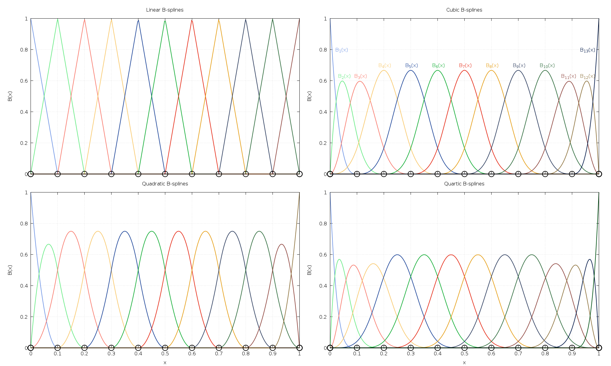
Fig. 40 Linear, quadratic, cubic, and quartic basis splines defined on the interval
with uniform knots. Black circles denote the location of
the knots.
This figure makes it clear that each B-spline has local support and spans
 knots. The B-splines near the interval endpoints appear to span
less knots, but note that the endpoint knots have multiplicities of .
knots. The B-splines near the interval endpoints appear to span
less knots, but note that the endpoint knots have multiplicities of .
The program is given below.
#include <stdio.h>
#include <stdlib.h>
#include <math.h>

#include <gsl/gsl_math.h>
#include <gsl/gsl_bspline.h>
#include <gsl/gsl_math.h>
#include <gsl/gsl_vector.h>

void
print_basis(FILE *fp_knots, FILE *fp_spline, const size_t order, const size_t nbreak)
{
  gsl_bspline_workspace *w = gsl_bspline_alloc(order, nbreak);
  const size_t p = gsl_bspline_ncontrol(w);
  const size_t n = 300;
  const double a = 0.0;
  const double b = 1.0;
  const double dx = (b - a) / (n - 1.0);
  gsl_vector *B = gsl_vector_alloc(p);
  size_t i, j;

  /* use uniform breakpoints on [a, b] */
  gsl_bspline_init_uniform(a, b, w);

  gsl_vector_fprintf(fp_knots, w->knots, "%f");

  for (i = 0; i < n; ++i)
    {
      double xi = i * dx;

      gsl_bspline_eval_basis(xi, B, w);

      fprintf(fp_spline, "%f ", xi);

      for (j = 0; j < p; ++j)
        fprintf(fp_spline, "%f ", gsl_vector_get(B, j));

      fprintf(fp_spline, "\n");
    }

  fprintf(fp_knots, "\n\n");
  fprintf(fp_spline, "\n\n");

  gsl_vector_free(B);
  gsl_bspline_free(w);
}

int
main (void)
{
  const size_t nbreak = 11; /* number of breakpoints */
  FILE *fp_knots = fopen("bspline1_knots.txt", "w");
  FILE *fp_spline = fopen("bspline1.txt", "w");

  print_basis(fp_knots, fp_spline, 2, nbreak); /* linear splines */
  print_basis(fp_knots, fp_spline, 3, nbreak); /* quadratic splines */
  print_basis(fp_knots, fp_spline, 4, nbreak); /* cubic splines */
  print_basis(fp_knots, fp_spline, 5, nbreak); /* quartic splines */

  fclose(fp_knots);
  fclose(fp_spline);

  return 0;
}
Example 2: Derivatives of Basis Splines
The following program computes and outputs cubic B-splines and their
derivatives using  breakpoints and uniform knots on the interval
. All derivatives up to order
breakpoints and uniform knots on the interval
. All derivatives up to order  are computed.
The output is shown in Fig. 41.
are computed.
The output is shown in Fig. 41.
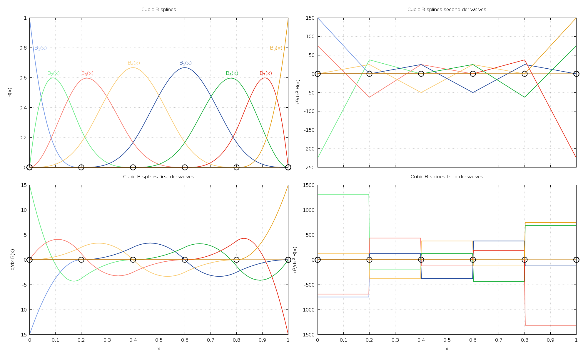
Fig. 41 Cubic B-splines and derivatives up to order 3. Black circles denote the location of the knots.
The program is given below.
#include <stdio.h>
#include <stdlib.h>
#include <math.h>

#include <gsl/gsl_math.h>
#include <gsl/gsl_matrix.h>
#include <gsl/gsl_bspline.h>

int
main (void)
{
  const size_t nbreak = 6;
  const size_t spline_order = 4;
  gsl_bspline_workspace *w = gsl_bspline_alloc(spline_order, nbreak);
  const size_t p = gsl_bspline_ncontrol(w);
  const size_t n = 300;
  const double a = 0.0;
  const double b = 1.0;
  const double dx = (b - a) / (n - 1.0);
  gsl_matrix *dB = gsl_matrix_alloc(p, spline_order);
  size_t i, j, k;

  /* uniform breakpoints on [a, b] */
  gsl_bspline_init_uniform(a, b, w);

  /* output knot vector */
  gsl_vector_fprintf(stdout, w->knots, "%f");
  printf("\n\n");

  for (i = 0; i < spline_order; ++i)
    {
      for (j = 0; j < n; ++j)
        {
          double xj = j * dx;

          gsl_bspline_eval_deriv_basis(xj, i, dB, w);

          printf("%f ", xj);

          for (k = 0; k < p; ++k)
            printf("%f ", gsl_matrix_get(dB, k, i));

          printf("\n");
        }

      printf("\n\n");
    }

  gsl_matrix_free(dB);
  gsl_bspline_free(w);

  return 0;
}
Example 3: Least squares and breakpoints
The following program computes a linear least squares fit to data using
cubic B-splines with uniform breakpoints. The data is generated from
the curve  with Gaussian noise added.
Splines are fitted with
with Gaussian noise added.
Splines are fitted with  and
and  breakpoints for comparison.
The program output is shown below:
$ ./a.out > bspline_lsbreak.txt
40 breakpoints: chisq/dof = 1.008999e+00
10 breakpoints: chisq/dof = 1.014761e+00
The data and fitted models are shown in Fig. 42.
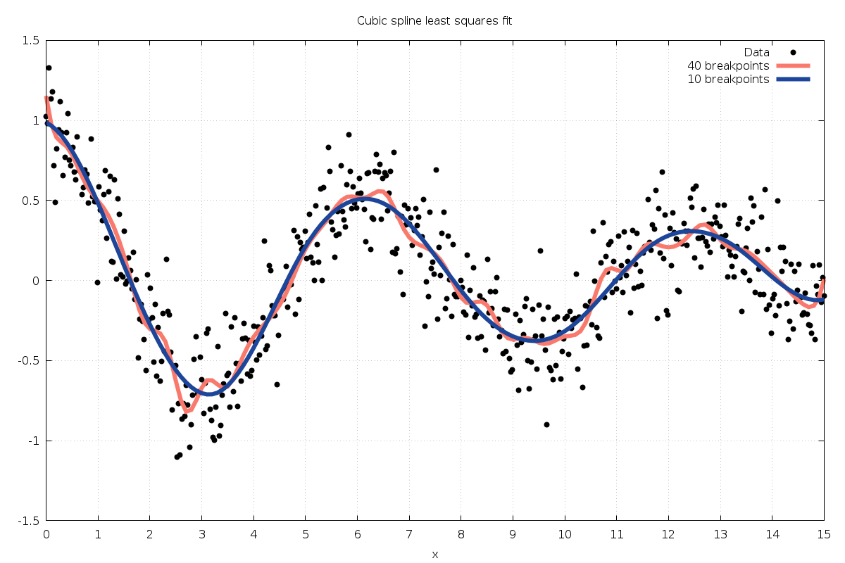
Fig. 42 Cubic B-spline least squares fit
The program is given below.
#include <stdio.h>
#include <stdlib.h>
#include <math.h>

#include <gsl/gsl_math.h>
#include <gsl/gsl_bspline.h>
#include <gsl/gsl_rng.h>
#include <gsl/gsl_randist.h>
#include <gsl/gsl_statistics.h>

int
main (void)
{
  const size_t n = 500;     /* number of data points to fit */
  const size_t k = 4;       /* spline order */
  const double a = 0.0;     /* data interval [a,b] */
  const double b = 15.0;
  const double sigma = 0.2; /* noise */
  gsl_bspline_workspace *work1 = gsl_bspline_alloc(k, 40);   /* 40 breakpoints */
  gsl_bspline_workspace *work2 = gsl_bspline_alloc(k, 10);   /* 10 breakpoints */
  const size_t p1 = gsl_bspline_ncontrol(work1);             /* number of control points */
  const size_t p2 = gsl_bspline_ncontrol(work2);             /* number of control points */
  const size_t dof1 = n - p1;                                /* degrees of freedom */
  const size_t dof2 = n - p2;                                /* degrees of freedom */
  gsl_vector *c1 = gsl_vector_alloc(p1);
  gsl_vector *c2 = gsl_vector_alloc(p2);
  gsl_vector *x = gsl_vector_alloc(n);
  gsl_vector *y = gsl_vector_alloc(n);
  gsl_vector *w = gsl_vector_alloc(n);
  size_t i;
  gsl_rng *r;
  double chisq1, chisq2;

  gsl_rng_env_setup();
  r = gsl_rng_alloc(gsl_rng_default);

  /* this is the data to be fitted */
  for (i = 0; i < n; ++i)
    {
      double xi = (b - a) / (n - 1.0) * i + a;
      double yi = cos(xi) * exp(-0.1 * xi);
      double dyi = gsl_ran_gaussian(r, sigma);

      yi += dyi;

      gsl_vector_set(x, i, xi);
      gsl_vector_set(y, i, yi);
      gsl_vector_set(w, i, 1.0 / (sigma * sigma));

      printf("%f %f\n", xi, yi);
    }

  /* use uniform breakpoints on [a, b] */
  gsl_bspline_init_uniform(a, b, work1);
  gsl_bspline_init_uniform(a, b, work2);

  /* solve least squares problem */
  gsl_bspline_wlssolve(x, y, w, c1, &chisq1, work1);
  gsl_bspline_wlssolve(x, y, w, c2, &chisq2, work2);

  fprintf(stderr, "40 breakpoints: chisq/dof = %e\n", chisq1 / dof1);
  fprintf(stderr, "10 breakpoints: chisq/dof = %e\n", chisq2 / dof2);

  printf("\n\n");

  /* output the spline curves */
  {
    double xi;

    for (xi = a; xi <= b; xi += 0.1)
      {
        double result1, result2;

        gsl_bspline_calc(xi, c1, &result1, work1);
        gsl_bspline_calc(xi, c2, &result2, work2);
        printf("%f %f %f\n", xi, result1, result2);
      }
  }

  gsl_rng_free(r);
  gsl_vector_free(x);
  gsl_vector_free(y);
  gsl_vector_free(w);
  gsl_vector_free(c1);
  gsl_vector_free(c2);
  gsl_bspline_free(work1);
  gsl_bspline_free(work2);

  return 0;
}
Example 4: Least squares and spline order
The following program computes least squares fits to the same
dataset in the previous example, using uniform
breakpoints and computing splines of order  .
.
The data and fitted models are shown in Fig. 43.
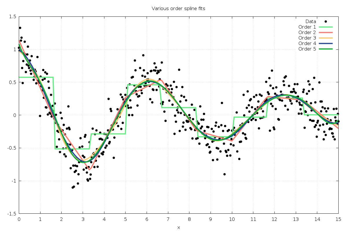
Fig. 43 B-spline least squares fit with varying spline orders
The program is given below.
#include <stdio.h>
#include <stdlib.h>
#include <math.h>

#include <gsl/gsl_math.h>
#include <gsl/gsl_bspline.h>
#include <gsl/gsl_rng.h>
#include <gsl/gsl_randist.h>
#include <gsl/gsl_statistics.h>

int
main (void)
{
  const size_t n = 500;              /* number of data points to fit */
  const double a = 0.0;              /* data interval [a,b] */
  const double b = 15.0;
  const size_t max_spline_order = 5; /* maximum spline order */
  const size_t nbreak = 10;          /* number of breakpoints */
  const double sigma = 0.2;          /* noise */
  gsl_bspline_workspace **work = malloc(max_spline_order * sizeof(gsl_bspline_workspace *));
  gsl_vector **c = malloc(max_spline_order * sizeof(gsl_vector *));
  gsl_vector *x = gsl_vector_alloc(n);
  gsl_vector *y = gsl_vector_alloc(n);
  gsl_vector *w = gsl_vector_alloc(n);
  size_t i;
  gsl_rng *r;
  double chisq;

  gsl_rng_env_setup();
  r = gsl_rng_alloc(gsl_rng_default);

  /* this is the data to be fitted */
  for (i = 0; i < n; ++i)
    {
      double xi = (b - a) / (n - 1.0) * i + a;
      double yi = cos(xi) * exp(-0.1 * xi);
      double dyi = gsl_ran_gaussian(r, sigma);

      yi += dyi;

      gsl_vector_set(x, i, xi);
      gsl_vector_set(y, i, yi);
      gsl_vector_set(w, i, 1.0 / (sigma * sigma));

      printf("%f %f\n", xi, yi);
    }

  printf("\n\n");

  for (i = 0; i < max_spline_order; ++i)
    {
      /* allocate workspace for this spline order */
      work[i] = gsl_bspline_alloc(i + 1, nbreak);
      c[i] = gsl_vector_alloc(gsl_bspline_ncontrol(work[i]));

      /* use uniform breakpoints on [a, b] */
      gsl_bspline_init_uniform(a, b, work[i]);

      /* solve least squares problem */
      gsl_bspline_wlssolve(x, y, w, c[i], &chisq, work[i]);
    }

  /* output the spline curves */
  {
    double xi;

    for (xi = a; xi <= b; xi += 0.1)
      {
        printf("%f ", xi);
        for (i = 0; i < max_spline_order; ++i)
          {
            double result;
            gsl_bspline_calc(xi, c[i], &result, work[i]);
            printf("%f ", result);
          }
        printf("\n");
      }
  }

  for (i = 0; i < max_spline_order; ++i)
    {
      gsl_vector_free(c[i]);
      gsl_bspline_free(work[i]);
    }

  gsl_rng_free(r);
  gsl_vector_free(x);
  gsl_vector_free(y);
  gsl_vector_free(w);
  free(work);
  free(c);

  return 0;
}
Example 5: Least squares, regularization and the Gram matrix
The following example program fits a cubic B-spline to data generated from the Gaussian

on the interval ![[-1.5,1.5]](_images/math/5b8fb2774bf010da025750345b5d78a394046efa.png) with noise added. Two data gaps are
deliberately introduced on
with noise added. Two data gaps are
deliberately introduced on ![[-1.1,-0.7]](_images/math/571ace076165f9edfc8e92915fd3c0abd2c5b0d3.png) and
and ![[0.1,0.55]](_images/math/9edc1617d6e5b9299bae122dddf83721982fb11e.png) ,
which makes the problem ill-posed. Fig. 44 shows
that the ordinary least squares solution exhibits large errors in
the data gap regions due to the ill-conditioned least squares matrix.
,
which makes the problem ill-posed. Fig. 44 shows
that the ordinary least squares solution exhibits large errors in
the data gap regions due to the ill-conditioned least squares matrix.
One way to correct the situation is to minimize the data misfit but also minimize the curvature of the spline averaged over the full interval. We can define the average curvature using the second derivative of the spline as follows:

where  is the Gram matrix of second derivatives of the B-splines.
Therefore, our regularized least squares problem is
is the Gram matrix of second derivatives of the B-splines.
Therefore, our regularized least squares problem is

where the regularization parameter  represents a tradeoff between
minimizing the data misfit and minimizing the spline curvature.
The solution of this least-squares problem is
represents a tradeoff between
minimizing the data misfit and minimizing the spline curvature.
The solution of this least-squares problem is

The example program below solves this problem without regularization  and with regularization
  for comparison. We also plot
the
for comparison. We also plot
the  confidence intervals for both solutions using the diagonal elements
of the covariance matrix
confidence intervals for both solutions using the diagonal elements
of the covariance matrix  .
.
Fig. 44 shows the result of regularizing the spline over the full interval, using the command
./a.out > data.txt
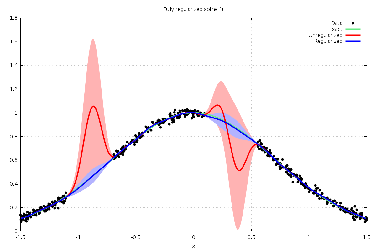
Fig. 44 B-spline least squares fit with exact (green), unregularized (red with confidence intervals),
and fully regularized (blue with confidence intervals) solutions.
Fig. 45 shows the result of regularizing the spline over the smaller
interval ![[0,0.6]](_images/math/8a2c3be58a5d1044c16d84f2d735113a712e8446.png) , correcting only the second gap, using the command
, correcting only the second gap, using the command
./a.out 0 0.6 > data.txt
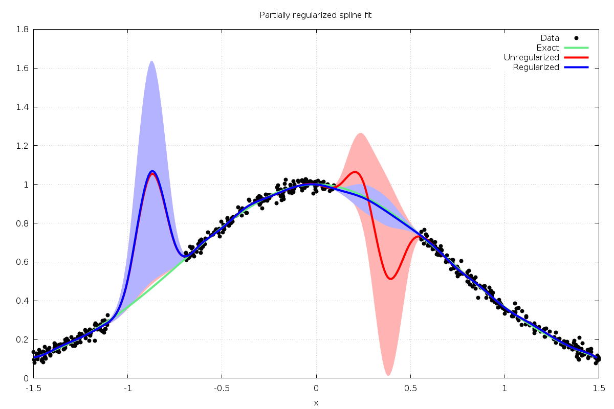
Fig. 45 B-spline least squares fit with exact (green), unregularized (red with confidence intervals),
and partially regularized (blue with confidence intervals) solutions.
The program is given below.
#include <stdio.h>
#include <stdlib.h>
#include <math.h>

#include <gsl/gsl_math.h>
#include <gsl/gsl_bspline.h>
#include <gsl/gsl_matrix.h>
#include <gsl/gsl_vector.h>
#include <gsl/gsl_linalg.h>
#include <gsl/gsl_rng.h>
#include <gsl/gsl_randist.h>

int
main (int argc, char * argv[])
{
  const size_t n = 500;                                     /* number of data points to fit */
  const size_t k = 4;                                       /* spline order */
  const double a = -1.5;                                    /* data interval [a,b] */
  const double b = 1.5;
  const double sigma = 0.02;                                /* noise */
  const double lambda_sq = 0.1;                             /* regularization parameter */
  gsl_bspline_workspace *work = gsl_bspline_alloc(k, 25);   /* 25 breakpoints */
  const size_t p = gsl_bspline_ncontrol(work);              /* number of control points */
  gsl_vector *c = gsl_vector_alloc(p);                      /* control points for unregularized model */
  gsl_vector *creg = gsl_vector_alloc(p);                   /* control points for regularized model */
  gsl_vector *x = gsl_vector_alloc(n);                      /* x data */
  gsl_vector *y = gsl_vector_alloc(n);                      /* y data */
  gsl_vector *w = gsl_vector_alloc(n);                      /* data weights */
  gsl_matrix *XTX = gsl_matrix_alloc(p, k);                 /* normal equations matrix */
  gsl_vector *XTy = gsl_vector_alloc(p);                    /* normal equations rhs */
  gsl_matrix *cov = gsl_matrix_alloc(p, p);                 /* covariance matrix */
  gsl_matrix *cov_reg = gsl_matrix_alloc(p, p);             /* covariance matrix for regularized model */
  gsl_matrix *G = gsl_matrix_alloc(p, k);                   /* regularization matrix */
  double reg_a = -1.0;                                      /* regularization interval [reg_a,reg_b] */
  double reg_b = -1.0;
  int reg_interval = 0;                                     /* apply regularization on smaller interval */
  size_t i;
  gsl_rng *r;

  if (argc > 2)
    {
      reg_a = atof(argv[1]);
      reg_b = atof(argv[2]);
      reg_interval = 1;
    }

  gsl_rng_env_setup();
  r = gsl_rng_alloc(gsl_rng_default);

  /* this is the data to be fitted */
  i = 0;
  while (i < n)
    {
      double ui = gsl_rng_uniform(r);
      double xi = (b - a) * ui + a;
      double yi, dyi;

      /* data gaps between [-1.1,-0.7] and [0.1,0.5] */
      if ((xi >= -1.1 && xi <= -0.7) || (xi >= 0.1 && xi <= 0.55))
        continue;

      dyi = gsl_ran_gaussian(r, sigma);
      yi = exp(-xi*xi) + dyi;

      gsl_vector_set(x, i, xi);
      gsl_vector_set(y, i, yi);
      gsl_vector_set(w, i, 1.0 / (sigma * sigma));

      printf("%f %f\n", xi, yi);

      ++i;
    }

  printf("\n\n");

  /* use uniform breakpoints on [a, b] */
  gsl_bspline_init_uniform(a, b, work);

  gsl_bspline_lsnormal(x, y, w, XTy, XTX, work); /* form normal equations matrix */
  gsl_linalg_cholesky_band_decomp(XTX);          /* banded Cholesky decomposition */
  gsl_linalg_cholesky_band_solve(XTX, XTy, c);   /* solve for unregularized solution */
  gsl_bspline_covariance(XTX, cov, work);        /* compute covariance matrix */

  /* compute regularization matrix */
  if (reg_interval)
    gsl_bspline_gram_interval(reg_a, reg_b, 2, G, work);
  else
    gsl_bspline_gram(2, G, work);

  /* multiply by lambda^2 */
  gsl_matrix_scale(G, lambda_sq);

  gsl_bspline_lsnormal(x, y, w, XTy, XTX, work);  /* form normal equations matrix */
  gsl_matrix_add(XTX, G);                         /* add regularization term */
  gsl_linalg_cholesky_band_decomp(XTX);           /* banded Cholesky decomposition */
  gsl_linalg_cholesky_band_solve(XTX, XTy, creg); /* solve for regularized solution */
  gsl_bspline_covariance(XTX, cov_reg, work);     /* compute covariance matrix */

  /* output the spline curves */
  {
    double xi;

    for (xi = a; xi <= b; xi += 0.01)
      {
        double result_unreg, result_reg;
        double err_unreg, err_reg;

        /* compute unregularized spline value and error at xi */
        gsl_bspline_calc(xi, c, &result_unreg, work);
        gsl_bspline_err(xi, 0, cov, &err_unreg, work);

        /* compute regularized spline value and error at xi */
        gsl_bspline_calc(xi, creg, &result_reg, work);
        gsl_bspline_err(xi, 0, cov_reg, &err_reg, work);

        printf("%f %e %e %e %e %e\n",
               xi,
               exp(-xi*xi),
               result_unreg,
               err_unreg,
               result_reg,
               err_reg);
      }
  }

  gsl_rng_free(r);
  gsl_vector_free(x);
  gsl_vector_free(y);
  gsl_vector_free(w);
  gsl_vector_free(c);
  gsl_vector_free(creg);
  gsl_bspline_free(work);
  gsl_matrix_free(XTX);
  gsl_vector_free(XTy);
  gsl_matrix_free(cov);
  gsl_matrix_free(cov_reg);
  gsl_matrix_free(G);

  return 0;
}
Example 6: Least squares and endpoint regularization
Data fitting with splines can often produce undesired effects at the spline
endpoints, where they are less constrained by data. As an example, we fit
order  splines to the Runge function,

with 20 uniform breakpoints on the interval ![[a,b] = [-1,1]](_images/math/1d53e8290434bdaf49584e0f83dc4119774a9397.png) .
Fig. 46 shows that the fitted spline (red) exhibits
a sharp upward feature at the left endpoint. This is due to the lack
of data constraining this part of the spline, and would likely result
in errors if the user wanted to extrapolate the spline outside the fit
interval. One method to correct this is to apply regularization to
the spline at the endpoints by minimizing one or more of its derivatives.
In this example, we minimize the first derivative of the spline at both
endpoints,
.
Fig. 46 shows that the fitted spline (red) exhibits
a sharp upward feature at the left endpoint. This is due to the lack
of data constraining this part of the spline, and would likely result
in errors if the user wanted to extrapolate the spline outside the fit
interval. One method to correct this is to apply regularization to
the spline at the endpoints by minimizing one or more of its derivatives.
In this example, we minimize the first derivative of the spline at both
endpoints,  and
and  . Note that

where  is the outer product matrix of first derivatives.
Therefore, our regularized least squares problem is
is the outer product matrix of first derivatives.
Therefore, our regularized least squares problem is

where we have chosen to use the same regularization parameter to regularize both
ends of the spline. In the example program below, we compute the unregularized solution ( )
and regularized solution (
)
and regularized solution ( ). The program outputs the first derivative of
the spline at both endpoints:
). The program outputs the first derivative of
the spline at both endpoints:
unregularized endpoint deriv 1: [ -1.081170e+01,  -2.963725e+00]
  regularized endpoint deriv 1: [ -2.735857e-02,  -5.371758e-03]
showing that the regularization has forced the first derivative smaller at both endpoints. The results are shown in Fig. 46.
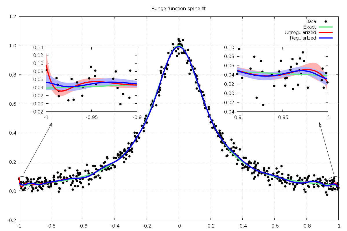
Fig. 46 Runge function B-spline least squares fit with exact (green), unregularized (red) and regularized (blue)
solutions. The zoomed inset views show the spline endpoints with confidence intervals.
The program is given below.
#include <stdio.h>
#include <stdlib.h>
#include <math.h>

#include <gsl/gsl_math.h>
#include <gsl/gsl_bspline.h>
#include <gsl/gsl_matrix.h>
#include <gsl/gsl_vector.h>
#include <gsl/gsl_linalg.h>
#include <gsl/gsl_rng.h>
#include <gsl/gsl_randist.h>

double
f(double x)
{
  return (1.0 / (1.0 + 25.0*x*x));
}

int
main (void)
{
  const size_t n = 500;                                     /* number of data points to fit */
  const size_t k = 10;                                      /* spline order */
  const double a = -1.0;                                    /* data interval [a,b] */
  const double b = 1.0;
  const double sigma = 0.03;                                /* noise */
  const double lambda_sq = 10.0;                            /* regularization parameter */
  const size_t nderiv = 1;                                  /* derivative order to regularize at endpoints */
  gsl_bspline_workspace *work = gsl_bspline_alloc(k, 20);   /* 20 breakpoints */
  const size_t p = gsl_bspline_ncontrol(work);              /* number of control points */
  gsl_vector *c = gsl_vector_alloc(p);                      /* control points for unregularized model */
  gsl_vector *creg = gsl_vector_alloc(p);                   /* control points for regularized model */
  gsl_vector *x = gsl_vector_alloc(n);                      /* x data */
  gsl_vector *y = gsl_vector_alloc(n);                      /* y data */
  gsl_vector *w = gsl_vector_alloc(n);                      /* data weights */
  gsl_matrix *XTX = gsl_matrix_alloc(p, k);                 /* normal equations matrix */
  gsl_vector *XTy = gsl_vector_alloc(p);                    /* normal equations rhs */
  gsl_matrix *cov = gsl_matrix_alloc(p, p);                 /* covariance matrix */
  gsl_matrix *cov_reg = gsl_matrix_alloc(p, p);             /* covariance matrix for regularized model */
  gsl_matrix *A1 = gsl_matrix_alloc(p, k);                  /* left regularization matrix */
  gsl_matrix *A2 = gsl_matrix_alloc(p, k);                  /* right regularization matrix */
  size_t i;
  gsl_rng *r;

  gsl_rng_env_setup();
  r = gsl_rng_alloc(gsl_rng_default);

  /* this is the data to be fitted */
  i = 0;
  while (i < n)
    {
      double ui = gsl_rng_uniform(r);
      double xi = (b - a) * ui + a;
      double yi, dyi;

      dyi = gsl_ran_gaussian(r, sigma);
      yi = f(xi) + dyi;

      gsl_vector_set(x, i, xi);
      gsl_vector_set(y, i, yi);
      gsl_vector_set(w, i, 1.0 / (sigma * sigma));

      printf("%f %f\n", xi, yi);

      ++i;
    }

  printf("\n\n");

  /* use uniform breakpoints on [a, b] */
  gsl_bspline_init_uniform(a, b, work);

  gsl_bspline_lsnormal(x, y, w, XTy, XTX, work); /* form normal equations matrix */
  gsl_linalg_cholesky_band_decomp(XTX);          /* banded Cholesky decomposition */
  gsl_linalg_cholesky_band_solve(XTX, XTy, c);   /* solve for unregularized solution */
  gsl_bspline_covariance(XTX, cov, work);        /* compute covariance matrix */

  /* compute regularization matrices */
  gsl_bspline_oprod(nderiv, a, A1, work);
  gsl_bspline_oprod(nderiv, b, A2, work);

  /* multiply by lambda^2 */
  gsl_matrix_scale(A1, lambda_sq);
  gsl_matrix_scale(A2, lambda_sq);

  gsl_bspline_lsnormal(x, y, w, XTy, XTX, work);  /* form normal equations matrix */
  gsl_matrix_add(XTX, A1);                        /* add regularization terms */
  gsl_matrix_add(XTX, A2);
  gsl_linalg_cholesky_band_decomp(XTX);           /* banded Cholesky decomposition */
  gsl_linalg_cholesky_band_solve(XTX, XTy, creg); /* solve for regularized solution */
  gsl_bspline_covariance(XTX, cov_reg, work);     /* compute covariance matrix */

  /* output the spline curves */
  {
    double xi;

    for (xi = a; xi <= b; xi += 0.001)
      {
        double result_unreg, result_reg;
        double err_unreg, err_reg;

        /* compute unregularized spline value and error at xi */
        gsl_bspline_calc(xi, c, &result_unreg, work);
        gsl_bspline_err(xi, 0, cov, &err_unreg, work);

        /* compute regularized spline value and error at xi */
        gsl_bspline_calc(xi, creg, &result_reg, work);
        gsl_bspline_err(xi, 0, cov_reg, &err_reg, work);

        printf("%f %e %e %e %e %e\n",
               xi,
               f(xi),
               result_unreg,
               err_unreg,
               result_reg,
               err_reg);
      }
  }

  {
    double result0, result1;

    gsl_bspline_calc_deriv(a, c, nderiv, &result0, work);
    gsl_bspline_calc_deriv(b, c, nderiv, &result1, work);
    fprintf(stderr, "unregularized endpoint deriv %zu: [%14.6e, %14.6e]\n", nderiv, result0, result1);

    gsl_bspline_calc_deriv(a, creg, nderiv, &result0, work);
    gsl_bspline_calc_deriv(b, creg, nderiv, &result1, work);
    fprintf(stderr, "  regularized endpoint deriv %zu: [%14.6e, %14.6e]\n", nderiv, result0, result1);
  }

  gsl_rng_free(r);
  gsl_vector_free(x);
  gsl_vector_free(y);
  gsl_vector_free(w);
  gsl_vector_free(c);
  gsl_vector_free(creg);
  gsl_bspline_free(work);
  gsl_matrix_free(XTX);
  gsl_vector_free(XTy);
  gsl_matrix_free(cov);
  gsl_matrix_free(cov_reg);
  gsl_matrix_free(A1);
  gsl_matrix_free(A2);

  return 0;
}
Example 7: Least squares and periodic splines
The following example program fits B-spline curves to a dataset which is periodic.
Both a non-periodic and periodic spline are fitted to the data for comparison. The
data is derived from the function on ![[0,2\pi]](_images/math/a72d3cd3c13fe84de3d730d119f7965720e2a8e1.png) ,
,

with Gaussian noise added. The program fits order  splines to the
dataset.
splines to the
dataset.
Fig. 47 Data (black) with non-periodic spline fit (red) and periodic spline fit (green).
The program additionally computes the derivatives up to order  at
the endpoints
at
the endpoints  and
and  :
:
=== Non-periodic spline endpoint derivatives ===
deriv 0: [ -8.697939e-01,  -8.328553e-01]
deriv 1: [ -2.423132e+00,   4.277439e+00]
deriv 2: [  3.904362e+01,   3.710592e+01]
deriv 3: [ -2.096142e+02,   2.036125e+02]
deriv 4: [  7.240121e+02,   7.384888e+02]
deriv 5: [ -1.230036e+03,   1.294264e+03]
=== Periodic spline endpoint derivatives ===
deriv 0: [ -1.022798e+00,  -1.022798e+00]
deriv 1: [  1.041910e+00,   1.041910e+00]
deriv 2: [  4.466384e+00,   4.466384e+00]
deriv 3: [ -1.356654e+00,  -1.356654e+00]
deriv 4: [ -2.751544e+01,  -2.751544e+01]
deriv 5: [  5.055419e+01,   2.674261e+01]
We can see that the periodic fit matches derivative values up
to order  , with the -th derivative being non-continuous.
The program is given below.
#include <stdio.h>
#include <stdlib.h>
#include <math.h>

#include <gsl/gsl_math.h>
#include <gsl/gsl_bspline.h>
#include <gsl/gsl_rng.h>
#include <gsl/gsl_randist.h>
#include <gsl/gsl_statistics.h>

int
main (void)
{
  const size_t n = 500;              /* number of data points to fit */
  const double a = 0.0;              /* data interval [a,b] */
  const double b = 2.0 * M_PI;
  const size_t spline_order = 6;     /* spline order */
  const size_t ncontrol = 15;        /* number of control points */
  const double sigma = 0.2;          /* noise */
  gsl_bspline_workspace *w = gsl_bspline_alloc_ncontrol(spline_order, ncontrol);
  gsl_bspline_workspace *wper = gsl_bspline_alloc_ncontrol(spline_order, ncontrol);
  gsl_vector *c = gsl_vector_alloc(ncontrol);    /* non-periodic coefficients */
  gsl_vector *cper = gsl_vector_alloc(ncontrol); /* periodic coefficients */
  gsl_vector *x = gsl_vector_alloc(n);
  gsl_vector *y = gsl_vector_alloc(n);
  gsl_vector *wts = gsl_vector_alloc(n);
  size_t i;
  gsl_rng *r;
  double chisq;

  gsl_rng_env_setup();
  r = gsl_rng_alloc(gsl_rng_default);

  /* this is the data to be fitted */
  for (i = 0; i < n; ++i)
    {
      double xi = (b - a) / (n - 1.0) * i + a;
      double yi = sin(xi) - cos(2.0 * xi);
      double dyi = gsl_ran_gaussian(r, sigma);

      yi += dyi;

      gsl_vector_set(x, i, xi);
      gsl_vector_set(y, i, yi);
      gsl_vector_set(wts, i, 1.0 / (sigma * sigma));

      printf("%f %f\n", xi, yi);
    }

  printf("\n\n");

  /* use uniform non-periodic knots on [a, b] */
  gsl_bspline_init_uniform(a, b, w);

  /* solve least squares problem for non-periodic spline */
  gsl_bspline_wlssolve(x, y, wts, c, &chisq, w);

  /* use periodic knots on [a, b] */
  gsl_bspline_init_periodic(a, b, wper);

  /* solve least squares problem for periodic spline */
  gsl_bspline_pwlssolve(x, y, wts, cper, &chisq, wper);

  /* output the spline curves */
  {
    double xi;

    for (xi = a; xi <= b; xi += 0.01)
      {
        double result, result_per;
        gsl_bspline_calc(xi, c, &result, w);
        gsl_bspline_calc(xi, cper, &result_per, wper);
        printf("%f %f %f\n", xi, result, result_per);
      }
  }

  fprintf(stderr, "=== Non-periodic spline endpoint derivatives ===\n");

  for (i = 0; i < spline_order; ++i)
    {
      double result0, result1;

      gsl_bspline_calc_deriv(a, c, i, &result0, w);
      gsl_bspline_calc_deriv(b, c, i, &result1, w);

      fprintf(stderr, "deriv %zu: [%14.6e, %14.6e]\n", i, result0, result1);
    }

  fprintf(stderr, "=== Periodic spline endpoint derivatives ===\n");

  for (i = 0; i < spline_order; ++i)
    {
      double result0, result1;

      gsl_bspline_calc_deriv(a, cper, i, &result0, wper);
      gsl_bspline_calc_deriv(b, cper, i, &result1, wper);

      fprintf(stderr, "deriv %zu: [%14.6e, %14.6e]\n", i, result0, result1);
    }

  gsl_vector_free(c);
  gsl_vector_free(cper);
  gsl_bspline_free(w);
  gsl_bspline_free(wper);
  gsl_rng_free(r);
  gsl_vector_free(x);
  gsl_vector_free(y);
  gsl_vector_free(wts);

  return 0;
}
Example 8: Projecting onto the B-spline basis
The following example program projects the function

onto a cubic B-spline basis with uniform knots on the interval ![[-2,2]](_images/math/69932d7e96401e5be702cfc25938a2f08b8af0b3.png) .
Because the function is cubic, it can be exactly decomposed in the B-spline basis.
.
Because the function is cubic, it can be exactly decomposed in the B-spline basis.
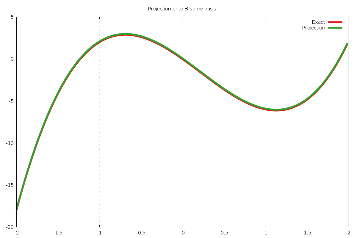
Fig. 48 Exact function (red) and spline projection (green). Small offset deliberately added to green curve.
The program is given below.
#include <stdio.h>
#include <stdlib.h>
#include <math.h>

#include <gsl/gsl_math.h>
#include <gsl/gsl_bspline.h>
#include <gsl/gsl_matrix.h>
#include <gsl/gsl_vector.h>
#include <gsl/gsl_linalg.h>

/* function to be projected */
double
f(double x, void * params)
{
  (void) params;
  return (x * (-7.0 + x*(-2.0 + 3.0*x)));
}

int
main (void)
{
  const size_t k = 4;                                       /* spline order */
  const double a = -2.0;                                    /* spline interval [a,b] */
  const double b = 2.0;
  gsl_bspline_workspace *work = gsl_bspline_alloc(k, 10);   /* 10 breakpoints */
  const size_t n = gsl_bspline_ncontrol(work);              /* number of control points */
  gsl_vector *c = gsl_vector_alloc(n);                      /* control points for spline */
  gsl_vector *y = gsl_vector_alloc(n);                      /* rhs vector */
  gsl_matrix *G = gsl_matrix_alloc(n, k);                   /* Gram matrix */
  gsl_function F;

  F.function = f;
  F.params = NULL;

  /* use uniform breakpoints on [a, b] */
  gsl_bspline_init_uniform(a, b, work);

  /* compute Gram matrix */
  gsl_bspline_gram(0, G, work);

  /* construct rhs vector */
  gsl_bspline_proj_rhs(&F, y, work);

  /* solve system */
  gsl_linalg_cholesky_band_decomp(G);
  gsl_linalg_cholesky_band_solve(G, y, c);

  /* output the result */
  {
    double x;

    for (x = a; x <= b; x += 0.01)
      {
        double result;
        gsl_bspline_calc(x, c, &result, work);
        printf("%f %f %f\n", x, GSL_FN_EVAL(&F, x), result);
      }
  }

  gsl_vector_free(y);
  gsl_vector_free(c);
  gsl_matrix_free(G);
  gsl_bspline_free(work);

  return 0;
}
Example 9: Interpolation
The following example program computes an interpolating cubic B-spline for a set of data. It constructs the collocation matrix for the dataset and factors it with a banded LU decomposition. The results are shown in Fig. 49.
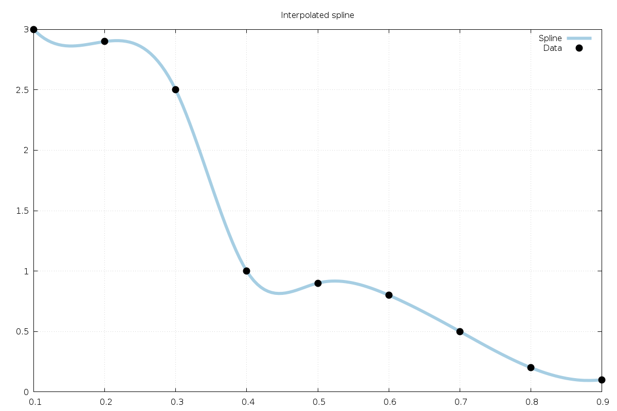
Fig. 49 Data points are shown in black and interpolated spline in light blue.
The program is given below.
#include <stdio.h>
#include <stdlib.h>
#include <math.h>

#include <gsl/gsl_math.h>
#include <gsl/gsl_bspline.h>
#include <gsl/gsl_matrix.h>
#include <gsl/gsl_vector.h>
#include <gsl/gsl_linalg.h>

int
main (void)
{
  const size_t n = 9;                  /* number of data to interpolate */
  const double x_data[] = { 0.1, 0.2, 0.3, 0.4, 0.5, 0.6, 0.7, 0.8, 0.9 };
  const double y_data[] = { 3.0, 2.9, 2.5, 1.0, 0.9, 0.8, 0.5, 0.2, 0.1 };
  gsl_vector_const_view xv = gsl_vector_const_view_array(x_data, n);
  gsl_vector_const_view yv = gsl_vector_const_view_array(y_data, n);
  const size_t k = 4;                                 /* spline order */
  gsl_vector *c = gsl_vector_alloc(n);                /* control points for spline */
  gsl_bspline_workspace *work = gsl_bspline_alloc_ncontrol(k, n);
  gsl_matrix * XB = gsl_matrix_alloc(n, 3*(k-1) + 1); /* banded collocation matrix */
  gsl_vector_uint * ipiv = gsl_vector_uint_alloc(n);
  double t;
  size_t i;

  /* initialize knots for interpolation */
  gsl_bspline_init_interp(&xv.vector, work);

  /* compute collocation matrix for interpolation */
  gsl_bspline_col_interp(&xv.vector, XB, work);

  /* solve linear system with banded LU */
  gsl_linalg_LU_band_decomp(n, k - 1, k - 1, XB, ipiv);
  gsl_linalg_LU_band_solve(k - 1, k - 1, XB, ipiv, &yv.vector, c);

  /* output the data */
  for (i = 0; i < n; ++i)
    {
      double xi = x_data[i];
      double yi = y_data[i];
      printf("%f %f\n", xi, yi);
    }

  printf("\n\n");

  /* output the spline */
  for (t = x_data[0]; t <= x_data[n-1]; t += 0.005)
    {
      double result;
      gsl_bspline_calc(t, c, &result, work);
      printf("%f %f\n", t, result);
    }

  gsl_vector_free(c);
  gsl_bspline_free(work);
  gsl_vector_uint_free(ipiv);
  gsl_matrix_free(XB);

  return 0;
}
References and Further Reading
Further information on the algorithms described in this section can be found in the following references,
C. de Boor, A Practical Guide to Splines (2001), Springer-Verlag, ISBN 0-387-95366-3.
L. L. Schumaker, Spline Functions: Basic Theory, 3rd edition, Cambridge University Press, 2007.
P. Dierckx, Algorithms for smoothing data with periodic and parametric splines, Computer Graphics and Image Processing, 20, 1982.
Dierckx, Curve and surface fitting with splines, Oxford University Press, 1995.
M. S. Mummy, Hermite interpolation with B-splines, Computer Aided Geometric Design, 6, 177–179, 1989.
Further information of Greville abscissae and B-spline collocation can be found in the following paper,
Richard W. Johnson, Higher order B-spline collocation at the Greville abscissae. Applied Numerical Mathematics. vol.: 52, 2005, 63–75.
A large collection of B-spline routines is available in the PPPACK library available at http://www.netlib.org/pppack, which is also part of SLATEC.