| [Top] | [Contents] | [Index] | [ ? ] |
| [ < ] | [ > ] | [ << ] | [ Up ] | [ >> ] | [Top] | [Contents] | [Index] | [ ? ] |
GNU Gama package is dedicated to adjustment of geodetic networks. It is intended for use with traditional geodetic surveyings which are still used and needed in special measurements (e.g., underground or high precision engineering measurements) where the Global Positioning System (GPS) cannot be used.
In general, surveying is the technique and science of accurately determining the terrestrial or three-dimensional spatial position of points and the distances and angles between them.(1)
Adjustment is a technical term traditionally used by geodesists and surveyors which simply means “application of the least squares method to process the over-determined system of measurements” (statistical methods other than least squares are used sometimes but are not common). In other words, we have more observations than needed and we are trying to get the best estimate for adjusted observations and/or coordinates.
Adjustment of geodetic networks means that we have a set of fixed points with given coordinates, a set of points with unknown coordinates (possibly with approximate values available) and a set of observations among them. What is typical of adjustment of special geodetic measurements is that the resulting linearized system might be singular (we can have a network with no fixed points) and we are not only interested in the values of ‘adjusted parameters and observations’ but also in the estimates of their covariances. This is what Gama does.
Gama was originally inspired by Fortran system Geodet/PC (1990) designed by Frantisek Charamza. The GNU Gama project started at the department of mapping and cartography, faculty of Civil Engineering, Czech Technical University in Prague (CTU) about 1998 and its name is an acronym for geodesy and mapping. It was presented to a wider public for the first time at FIG Working Week 2000 in Prague and then at FIG Workshop and Seminar at HUT Helsinki in 2001.
The GNU Gama home page is
http://www.gnu.org/software/gama/
and the project is hosted on
http://savannah.gnu.org/git/?group=gama
GNU Gama is released under the GNU General Public License and is based
on a C++ library of geodetic classes and functions and a small C++
template matrix library matvec. For parsing XML documents GNU
Gama calls the expat parser version 1.1, written by James
Clark. The expat parser is not part of the GNU Gama project,
but it is used by the project.
Adjustment in local Cartesian coordinate systems is fully supported
by a command-line program gama-local that adjusts geodetic
(free) networks of observed distances, directions, angles, height
differences, 3D vectors and observed coordinates (coordinates with
given variance-covariance matrix). Adjustment in global coordinate
systems is supported only partly as a gama-g3 program.
| 1.1 Download | ||
| 1.2 Install | ||
1.3 Program gama-local | ||
| 1.4 Reporting bugs | ||
| 1.5 Contributors |
| [ < ] | [ > ] | [ << ] | [ Up ] | [ >> ] | [Top] | [Contents] | [Index] | [ ? ] |
GNU Gama can be found in the subdirectory /gnu/gama/ on
your favourite FTP GNU mirror or
cloned from the GIT. See our project page at
savannah for more
information.
To get anonymous read-only access to the GIT repository for the latest GNU Gama source, issue the following command
git clone git://git.sv.gnu.org/gama.git |
| [ < ] | [ > ] | [ << ] | [ Up ] | [ >> ] | [Top] | [Contents] | [Index] | [ ? ] |
GNU Gama is developed and tested under GNU/Linux. A static library
libgama.lib and executables are build in folders lib and
src. You can compile Gama easily yourself if you download the
sources from a FTP server. The preferred way is to have expat
XML parser installed on your system, if not, GNU Gama will be build
with internally stored expat older source codes version 1.1.
Change to the directory of Gama project and issue the following commands at the shell prompt (with some optional parameters)
$ ./configure [--enable-extra-tests --bindir=DIR --infodir=DIR] $ make |
For GNU Gama test suite run
$ make check |
If the script configure is not available (which is the
case when you download source codes from the
git server), you have to
generate it using auxiliary script autogen.sh. To compile and
build all binaries. Run
$ ./autogen.sh $ ./configure |
and
$ make install [--prefix=/your/prefered/install/directory] |
if you also want to install executables and info documentation.
Typically, if you want to download (see section Download) and compile sources, you will run following commands:
$ git clone git://git.sv.gnu.org/gama.git gama $ cd gama $ ./autogen.sh $ ./configure $ make |
You should have expat XML parser and SQLite library already installed
on your system.
For example to be able to compile Gama on Ubuntu 10.04 you have to install
following packages:
make doxygen git automake autoconf libexpat1-dev libsqlite3-dev |
To compile user documentation in various formats (PDF, HTML, …) run the following commands
$ cd doc/ $ make download-gendocs.sh $ make run-gendocs.sh |
The documentation should be in doc/manual directory.
To compile API documentation run
$ doxygen |
in your gama directory.
Doxygen output will be in the doxygen directory.
| 1.2.1 CMake | ||
| 1.2.2 pkgsrc | ||
| 1.2.3 Precompiled executables for Windows |
| [ < ] | [ > ] | [ << ] | [ Up ] | [ >> ] | [Top] | [Contents] | [Index] | [ ? ] |
Alternatively you can use CMake to generate makefiles for Unix,
Windows, Mac OS X, OS/2, MSVC, Cygwin, MinGW or Xcode. Configuration
file CMakeLists.txt is available from the root distribution
directory. For example to build gama-local binary for Linux run
$ mkdir build_dir $ cd build_dir $ cmake .. [ -G generator-name ] $ make --build . |
where build_dir is an arbitrary directory name for
out-of-place build and optional generator-name specifies
a build system generator, for example Ninja.
| [ < ] | [ > ] | [ << ] | [ Up ] | [ >> ] | [Top] | [Contents] | [Index] | [ ? ] |
pkgsrc is a framework for managing third-party software on
UNIX-like systems, currently containing over 26,000 packages. It is
the default package manager of NetBSD and SmartOS, and can be used to
enable freely available software to be built easily on a large number
of other UNIX-like platforms. The binary packages that are produced by
pkgsrc can be used without having to compile anything from source. It
can be easily used to complement the software on an existing system.
Gama is available via pkgsrc as geography/gama, see https://www.pkgsrc.org/ for more information.
| [ < ] | [ > ] | [ << ] | [ Up ] | [ >> ] | [Top] | [Contents] | [Index] | [ ? ] |
qgama is a Qt application for adjustment of geodetic networks
with database support, where the database can be a simple SQLite3 flat
file, used for storing geodetic network data, or any full-featured
relational DBMS with Qt driver available like PostgreSQL or MySQL. It
is build on the GNU gama adjustment library.
Windows executable qgama.exe with all DLL libraries is
available from the GNU FTP server
https://ftp.gnu.org/gnu/gama/windows/
together with command-line interface executables gama-local.exe
and gama-g3 in the subdirectory bin.
| [ < ] | [ > ] | [ << ] | [ Up ] | [ >> ] | [Top] | [Contents] | [Index] | [ ? ] |
gama-localProgram gama-local is a simple command line tool for adjustment
of geodetic free networks. It is available for GNU Linux (the
main platform on which project GNU Gama is being developed), BSD or
Windows.
Program gama-local reads input data in XML format (XML input data format for gama-local) and prints adjustment results into
ASCII text file. If output file name is not given, adjustment results
in XML format are sent to the standard output device.
If development files for Sqlite3 (package libsqlite3-dev) are
installed, gama-local also supports reading
adjustment input data from sqlite3 database.
When run without arguments gama-local [--help]
prints a review of runtime options
Adjustment of local geodetic network        version: 2.29
************************************
https://www.gnu.org/software/gama/

Usage: gama-local  [--input-xml] input.xml  [options]
       gama-local  [--input-xml] input.xml  --sqlitedb sqlite.db  --configuration name  [options]
       gama-local  --sqlitedb sqlite.db  --configuration name  [options]
       gama-local  --sqlitedb sqlite.db  --readonly-configuration name  [options]

Options:

--algorithm  gso | svd | cholesky | envelope
--language   en | ca | cz | du | es | fi | fr | hu | ru | ua | zh
--encoding   utf-8 | iso-8859-2 | iso-8859-2-flat | cp-1250 | cp-1251
--angular    400 | 360
--latitude   <latitude>
--ellipsoid  <ellipsoid name>
--text       adjustment_results.txt
--html       adjustment_results.html
--xml        adjustment_results.xml
--octave     adjustment_results.m
--svg        network_configuration.svg
--cov-band   covariance matrix of adjusted parameters in XML output
             n  = -1  for full covariance matrix (implicit value)
             n >=  0  covariances are computed only for bandwidth n
--iterations maximum number of iterations allowed in the linearized
             least squares algorithm (implicit value is 5)
--export     updated input data based on adjustment results
--verbose    [yes | no]
--version
--help

Report bugs to: <bug-gama@gnu.org>
GNU gama home page: <https://www.gnu.org/software/gama/>
General help using GNU software: <https://www.gnu.org/gethelp/>
|
Program version is followed by information on
compiler used to build the program (apart from GNU g++
compiler other possibilities are Clang, Intel C++ compiler and
Visual C++, when build under Microsoft Windows).
Program gama-local can read XML input from the standard input
if you put "-" (hyphen) after the option --input-xml. This
option is special because it is optional (you can specify XML input
file name or "-" without it). Elective --input-xml enables
backward compatibility with the usage of older versions.
Adjustment results (--text, --xml) and others can be
similarly redirected to standard output if instead of a file name is
used "-" string. If no output is given, XML adjustment format is
implicitly send to standard output.
Option --algorithm enables to select numerical method for
solution of the adjustment.
Implicit algorithm is sparse matrix envelope.
Another possibilities are
Cholesky decomposition of semidefinite matrix of normal
equations (cholesky),
block matrix algorithm GSO by Frantisek Charamza based on
Gram-Schmidt orthogonalization (gso) and
Singular Value Decomposition (svd).
In the last two cases (gso and svd) project equations
are solved directly without forming normal equations.
Option --language selects language used in output protocol. For
example, if run with option --language cz, gama-local
prints output results in Czech languague using UTF-8
encoding. Implicit value is en for output in English.
Option --encoding enables to change inplicit UTF-8 output
encoding to iso-8859-2 (latin-2), iso-8859-2-flat (latin-2 without
diacritics), cp-1250 (MS-EE encoding) cp-12251 (Russian encoding).
Option --angular selects angular units to be used in output.
Options --latitude and/or --ellipsoid are used when
observed vertical and/or zenith angles need to be transformed into the
projection plane. If none of these two options is explicitly used, no
corrections are added to horizontal and/or zenith angles. If only one
of these options is used, then implicit value for --latitude is
45 degrees (50 gons) and implicit ellipsoid is WGS84.
Mathematical formulas for the corrections is given in the following
section.
Option --octave is used to output simplified adjustment results
for GNU Octave, i.e. in
an .m file. The following information is give in the output
file
In the case of free networks system of normal equations is augmented
with matrix of constrains. Adjustmment can be then computed
independetly in Octave and compared with results from Gama for unknown
coordinates. We suggest that for comaprision of Gama and Octave
results number of itereations is set to zero (--iterations 0).
This Octave output is currently available only for algorithm envelope (Gama version 2.10), also adjustment in Octave is not supported for the special case of one fixed point and one constrained (where normal equation cannot be directly augmented with constraints because of different number of unknowns).
Option --cov-band is used to reduce the number of computed
covariances (cofactors) in XML adjustment output. Implicitly full
matrix is written to XML output, which could degrade time efficiency
for the envelope algorithm for sparse matrix solution. Explicit
option for full covariance matrix is --cov-band -1, option
--cov-band 0 means that only a diagonal of covariance matrix is
written to XML output, --cov-band 1 results in computing the
main diagonal and first codiagonal etc. If higher rank is specified then
available, it is reduced do maximum possible value dim-1.
Option --iterations enables to set maximum number of
iterations allowed in the linearized least squares algorithm. After
the adjustment gama-local computes differences between adjusted
observations computed from residuals and from adjusted coordinates. If
the positional difference is higher than 0.5mm, approximate
coordinates of adjusted points are updated and the whole adjustment is
repeated in a new iteration. Implicit number of iterations is 5.
| 1.3.1 Reductions of horizontal and zenith angles |
| [ < ] | [ > ] | [ << ] | [ Up ] | [ >> ] | [Top] | [Contents] | [Index] | [ ? ] |
For evaluating of reductions of horizontal and zenith angles,
gama-local computes a helper point P_1 in the center of
the network. Horizontal and zenith angles observed at point P_2
are transformed to the projection plane perpendicular to the normal
z_1 of the helper point P_1. Coordinates (x_2,
y_2) of point P_2 are conserved, but its normal z_2 is
rotated by the central angle 2\gamma_12 to be parallel with
z_1.
Formulas for reductions of horizontal and zenith angles are given only in the printed version.
| [ < ] | [ > ] | [ << ] | [ Up ] | [ >> ] | [Top] | [Contents] | [Index] | [ ? ] |
Undoubtedly there are numerous bugs remaining, both in the C++ source code and in the documentation. If you find a bug in either, please send a bug report to
We will try to be as quick as possible in fixing the bugs and redistributing the fixes. If you prefere, you can always write directly to Aleš Čepek.
| [ < ] | [ > ] | [ << ] | [ Up ] | [ >> ] | [Top] | [Contents] | [Index] | [ ? ] |
The following persons (in chronological order) have made contributions to GNU Gama project: Aleš Čepek, Jiří Veselý, Petr Doubrava, Jan Pytel, Chuck Ghilani, Dan Haggman, Mauri Väisänen, John Dedrum, Jim Sutherland, Zoltan Faludi, Diego Berge, Boris Pihtin, Stéphane Kaloustian, Siki Zoltan, Anton Horpynich, Claudio Fontana, Bronislav Koska, Martin Beckett, Jiří Novák, Václav Petráš, Jokin Zurutuza, 项维 (Vim Xiang), Tomáš Kubín, Greg Troxel, Kristian Evers, Oleg Goussev, Petra Millarová, Jan Holešovský and Friedhelm Krumm.
Jiří Veselý is the author of calculation of approximate coordinates by
intersections and transformations (class Acord).
Václav Petráš is the author of SQL schema, SQLite and gama-local.
Petra Millarová is the main author of class Acord2 and other helper
classes for combinatorial solution of medians of approximate
coordinates.
Friedhelm Krumm, Geodätisches Institut Universität Stuttgart,
contributed numerical examples for the adjustment of geodetic networks
(1D, 2D and 3D) published in his Geodetic Network Adjustment Examples,
Rev. 3.5, January 20, 2020. https://www.gis.uni-stuttgart.de/
In version 2.18 the format of input data used in his Examples
was implemented in GNU Gama and is used in command line conversion
program gama-local-krumm2xml and also directly in qgama
GUI.
| [ < ] | [ > ] | [ << ] | [ Up ] | [ >> ] | [Top] | [Contents] | [Index] | [ ? ] |
gama-localThe input data format for a local geodetic network adjustment (program
gama-local) is defined in accordance with the definition of Extended
Markup Language (XML) for description of structured data.
The XML definition can be found at
Input data (points, observations and other related information) are
described using XML start-end pair tags <xxx> and </xxx>
and empty-element tags <xxx/>.
The syntax of XML gama-local input format is described in XML
schema (XSD), the file gama-local.xsd is a part of the
GNU gama distribution and can formally be validated
independently on the program gama-local, namely in unit testing
we use xmllint validating parser, if it is installed.
For parsing the XML input data, gama-local uses the XML parser
Expat copyrighted by James Clark which is described at
http://www.jclark.com/xml/expat.html
Expat is subject to the Mozilla Public License (MPL), or may
alternatively be used under the GNU General Public License (GPL)
instead.
In the gama-local XML input, distances are given in meters,
angular values in centigrades and their standard deviations (rms
errors) in millimeters or centigrade seconds, respectively.
Alternatively angular values in gama-local XML input can be
given in degrees and seconds (see section Angular units). At the end of
this chapter an example of the gama-local XML input data
object is given.
| 2.1 Angular units | ||
| 2.2 Prologue | XML declaration | |
2.3 Tags <gama-local> and <network> | ||
| 2.4 Network description | Tag <description>
| |
| 2.5 Network parameters | Tag <parameters />
| |
| 2.6 Points and observations | Tag <points-observations>
| |
| 2.7 Points | Tag <point />
| |
| 2.8 Set of observations | Tag <obs>
| |
| 2.9 Directions | Tag <direction />
| |
| 2.10 Horizontal distances | Tag <distance />
| |
| 2.11 Angles | Tag <angle />
| |
| 2.12 Slope distances | Tag <s-distance />
| |
| 2.13 Zenith angles | Tag <z-angle />
| |
| 2.14 Azimuths | Tag <azimuth />
| |
| 2.15 Height differences | Tag <height-differences>
| |
| 2.16 Control coordinates | Tag <coordinates>
| |
| 2.17 Coordinate differences (vectors) | Tag <vectors>
| |
2.18 Attribute extern | ||
| 2.19 Example of local geodetic network | A complete example of a network |
| [ < ] | [ > ] | [ << ] | [ Up ] | [ >> ] | [Top] | [Contents] | [Index] | [ ? ] |
Horizontal angles, directions and zenith angles in gama-local
XML adjustment input are implicitly given in gons and their standard
deviations and/or variances in centicentigons. Gon, also called
centesimal grade and Neugrad (German for new grad), is 1/400-th of the
circumference. For example
<direction from="202" to="416" val="63.9347" stdev="10.0" /> |
The same angular value (direction) can be expressed in degrees (sexagesimal graduation) as
<direction from="202" to="416" val="57-32-28.428" stdev="3.24" /> |
In XML adjustment input degrees are coded as a single string, where degrees (57), minutes (32) and seconds (28.428) are separated by dashes (-) with optional leading sign. Spaces are not allowed inside the string. Gons and degrees may be mixed in a single XML document but one should be careful to supply the information on standard deviations and/or covariances in the proper corresponding units.
Sexagesimal seconds (ss) are commonly called arcseconds, they are related to the metric system centicentigons (cc) as
ss = cc/400/100/100 * 360*60*60 = cc*0.324.
Internally gama-local works with gons but output can be
transformed to degrees using the option --angular 360.
Another angular unit commonly used in surveying is the milligon (mgon), 1 mgon = 1 gon/1000 (similarly as 1 mm = 1 m/1000) and 10 cc = 1 mgon.
| [ < ] | [ > ] | [ << ] | [ Up ] | [ >> ] | [Top] | [Contents] | [Index] | [ ? ] |
XML documents begin with an XML declaration that specifies the version
of XML being used (prolog). In the case of gama-local
follows the root tag <gama-local> with XML Schema namespace
defined in attribute xmlns:
<?xml version="1.0" ?> <gama-local xmlns="http://www.gnu.org/software/gama/gama-local"> |
GNU Gama uses non-validating parser and the XML Schema Definition
namespace is not used in gama-local but it is essential for
usage in third party software that might need XML validation.
| [ < ] | [ > ] | [ << ] | [ Up ] | [ >> ] | [Top] | [Contents] | [Index] | [ ? ] |
<gama-local> and <network>A pair tag <gama-local> contains a single pair tag <network>
that contains the network definition. The definition of the network is
composed of three sections:
<description> of the network (annotation or comments),
<parameters /> and
<points-observations> section.
The sections <description> and <parameters /> are
optional, the section <points-observations> is mandatory. These
three sections may be presented in any order and may be repeated several
times (in such a case, the corresponding sections are linked
together by the software).
The pair tag <network> has two optional attributes axes-xy
and angles. These attributes are used to describe orientation of
the xy orthogonal coordinate system axes and the orientation of the
observed angles and/or directions.
axes-xy="ne" orientation of axes x and y; value
ne implies that axis x is oriented north and axis y
is oriented east. Acceptable values are ne, sw,
es, wn for left-handed coordinate systems and en,
nw, se, ws for right-handed coordinate systems
(default value is ne).
angles="right-handed" defines counterclockwise observed angles
and/or directions, value left-handed defines clockwise observed
angles and/or directions (default value is left-handed).
Many geodetic systems are right handed with x axis oriented
east, y axis oriented north and counterclockwise angular
observations. Example of left-handed orthogonal system with different
axes orientation is coordinate system Krovak used in the Czech
Republic where the axes x and y are oriented south and
west respectively.
GNU Gama can adjust any combination of coordinate and angular systems.
<gama-local> <network> <description> ... </description> <parameters ... /> <points-observations> ... </points-observations> </network> </gama-local> |
It is planned in future versions of the program to allow more
<network> tags (analysis of deformations etc.) and definitions of
new tags.
| [ < ] | [ > ] | [ << ] | [ Up ] | [ >> ] | [Top] | [Contents] | [Index] | [ ? ] |
The description of a geodetic network is enclosed in the start-end pair
tags <description>. Text of the description is copied into the
adjustment output and serves for easier identification of results. The
text is not interpreted by the program, but it may be helpful for users.
<description> A short description of a geodetic network ... </description> |
| [ < ] | [ > ] | [ << ] | [ Up ] | [ >> ] | [Top] | [Contents] | [Index] | [ ? ] |
The network parameters may be listed with the following optional
attributes of an empty-element tag <parameters />
sigma-apr = "10" value of a priori reference standard
deviation—square root of reference variance (default value 10)
conf-pr = "0.95" confidence probability used in statistical
tests (dafault value 0.95)
tol-abs = "1000" tolerance for identification of gross
absolute terms in project equations (default value 1000 mm)
sigma-act = "aposteriori" actual type of reference standard deviation
use in statistical tests (aposteriori | apriori); default value
is aposteriori
algorithm = "gso" numerical algortihm used in the adjistment
(gso, svd, cholesky, envelope).
languade = "en" the language to be used in adjustment output.
encoding = "utf-8" adjustment output encoding.
angular = "400" output results angular units (400/360).
latitude = "50"
ellipsoid
cov-band = "-1" the bandwith of covariance matrix of the
adjusted parameters in the output XML file (-1 means all covariances).
Values of the attributes must be given either in the double-quotes
("…") or in the single quotes ('…'). There
can be white spaces (spaces, tabs and new-line characters)
between attribute names, values, and the equal sign.
<parameters sigma-apr = "15"
            conf-pr   = '0.90'
            sigma-act = "apriori" />
|
| [ < ] | [ > ] | [ << ] | [ Up ] | [ >> ] | [Top] | [Contents] | [Index] | [ ? ] |
The points and observations section is bounded by the pair tag
<points-observations> and contains information about points,
observed horizontal directions, angles, and horizontal distances, height
differences, slope distances, zenith angles, observed vectors and
control coordinates.
Optional attributes of the start tag <points-observations> allow
for the definition of default values of standard deviations
corresponding to observed directions, angles, and distances.
direction-stdev = "…" defines the implicit value of
standard deviation of observed directions (default value is not
defined)
angle-stdev = "…" defines the implicit value of standard
deviation of observed angles (default value is not defined)
zenith-angle-stdev = "…" defines the implicit value of
standard deviation of observed zenith angles (default value is not
defined)
azimuth-stdev = "…" defines the implicit value of
standard deviation of observed azimuth angles (default value is not
defined)
distance-stdev = "…" defines the implicit value of
standard deviation of observed distances, horizontal or slope (default
value is not defined)
Implicit values of standard deviations for the observed distances are calculated from the model with three constants a, b, and c according to the formula
a + bD^c,
where a is a constant part of the model and D is the observed distance in kilometres. If the constants b and/or c are not given, default values b=0 and c=1 will be used.
<points-observations direction-stdev = "10"
                     distance-stdev  = "5 3 1" >
   <!-- ... points and observation data ... -->
</points-observations>
|
| [ < ] | [ > ] | [ << ] | [ Up ] | [ >> ] | [Top] | [Contents] | [Index] | [ ? ] |
Points are described by the empty-element tags <point/> with the
following attributes:
id = "…" is the point identification attribute (mandatory);
point identification is not limited to numbers; all printable
characters can be used in identification.
x = "…" specifies coordinate x
y = "…" specifies coordinate y
z = "…" specifies coordinate z, point height
fix = "…" specifies coordinates that are fixed in
adjustment; acceptable values are xy, XY, z,
Z, xyz, XYZ, xyZ and XYz.
adj = "…" specifies coordinates to be adjusted (unknown
parameters in adjustment); acceptable values are xy, XY,
z, Z, xyz, XYZ, xyZ and XYz.
With exception of the first attribute (point id), all other attributes are optional. Decimal numbers can be used as needed.
Control coordinates marked using the fix parameter are not
changed in the adjustment. Uppercase and lowercase notation of
coordinates with the fix parameter are interpreted the same.
Corrections are applied to the unknown parameters identified by
coordinates written in lowercase characters given in the adj
parameter. When the coordinates are written using uppercase, they are
interpreted as constrained coordinates. If coordinates are marked
with both the fix and adj, the fix parameter will
take precedence.
Constrained coordinates are used for the regularization of free networks. If the network is not free (fixed network), the constrained coordinates are interpreted as other unknown parameters. In classical free networks, the constrained points define the regularization constraint
\sum dx^2_i+dy^2_i = \min.
where dx and dy are adjusted coordinate corrections and
the summation index i goes over all constrained points.
In other words, the set of the constrained points defines the
adjustment of the free network (its shape and size) with a
simultaneous transformation to the approximate coordinates of selected
points. Program gama-local allows the definition of
constrained coordinates with 1D leveling networks, 2D and 3D local
networks.
<point id="1" y="644498.590" x="1054980.484" fix="xy" /> <point id="2" y="643654.101" x="1054933.801" adj="XY" /> <point id="403" adj="xy" /> |
| [ < ] | [ > ] | [ << ] | [ Up ] | [ >> ] | [Top] | [Contents] | [Index] | [ ? ] |
The pair tag <obs> groups together a set of observations which
are somehow related. A typical example is a set of directions and
distances observed from one stand-point. An observation section
contains a set of
<direction … />
<distance … />
<angle … />
<s-distance … />
<z-angle … />
<azimuth … />
The band variance-covariance matrix of directions, distances, angles
or other observations
listed in one <obs> section may be supplied using a
<cov-mat> pair tag with attributes dim (dimension) and
band (bandwidth). The band-width of the diagonal matrix is equal
to 0 and a fully-populated variance-covariance matrix has a bandwidth of
dim-1.
Observation variances and covariances (i.e. an upper-symmetric part of
the band-matrix) are written row by row between <cov-mat> and
</cov-mat> tags. If present, the dimension of the
variance-covariance matrix must agree with the number of observations.
The following example of variance-covariance matrix with dimension 6 and bandwidth 2 (two nonzero codiagonals and three zero codiagonals)
[ 1.1 0.1 0.2 0 0 0 0.1 1.2 0.3 0.4 0 0 0.2 0.3 1.3 0.5 0.6 0 0 0.4 0.5 1.4 0.7 0.8 0 0 0.6 0.7 1.5 0.9 0 0 0 0.8 0.9 1.6 ] |
is coded in XML as
<cov-mat dim="6" band="2">
   1.1  0.1  0.2
        1.2  0.3  0.4
             1.3  0.5  0.6
                  1.4  0.7  0.8
                       1.5  0.9
                            1.6
</cov-mat>
|
If two or more sets of directions with different orientations are
observed from a stand-point, they must be placed in different <obs>
sections. The value of an orientation angle can be explicitly stated
with an attribute orientation="…". Normally, it is more
convenient to let the program calculate approximate values of
orientations needed for the adjustment. If directions are present, then
the attribute station must be defined.
Optional attribute from_dh="…" enables to enter implicit
height of instrument for all observations within the <obs> pair
tag.
Observed distances are expressed in meters, their standard deviations in millimeters. Observed directions and angles are expressed in centigrades (400) and their standard deviations in centigrade seconds.
<obs from="418">
   <direction  to=  "2" val="0.0000"   stdev="10.0" />
   <direction  to="416" val="63.9347"  stdev="10.0" />
   <direction  to="420" val="336.3190" stdev="10.0" />
   <distance   to="420" val="246.594"  stdev="5.0"  />
</obs>

<obs from="418">
   <direction  to=  "2" val="0.0000"   />
   <direction  to="416" val="63.9347"  />
   <direction  to="420" val="336.3190" />
   <distance   to="420" val="246.594"  />

   <cov-mat dim="4" band="0">
      100.00 100.00 100.00 25.00
   </cov-mat>
</obs>
|
| [ < ] | [ > ] | [ << ] | [ Up ] | [ >> ] | [Top] | [Contents] | [Index] | [ ? ] |
Directions are expressed with the following attributes in an
empty-element tag <direction />
to = "…" target point identification
val = "…" observed direction; see section Angular units
stdev = "…" standard deviation (optional)
from_dh = "…" instrument height (optional)
to_dh = "…" reflector/target height (optional)
The standard deviation is an optional attribute. However since all
observations in the adjustment must have their weights defined, the
standard deviation must be given either explicitly with the attribute
stdev="…" or implicitly with <points-observation
direction-stdev="…" > or with a variance-covariance matrix for
the given observation set. A similar approach applies to all the
observations (distances, angles, etc.)
All directions in the given <obs> tag (see section Set of observations) share a common orientation shift, which is an
implicit adjustment unknown parameter defining relation between the
stand point directions and bearings
direction_AB + orientation shift_A = bearing_AB.
Because one <obs> tag defines one orientation shift for all its
directions, stand point id must be given in the <obs
from="id"> tag, using attribute from, which in turn must not be
used in <direction /> tags, to avoid unintentional discrepancies.
<direction to= "2" val="0.0000" stdev="10.0" /> <direction to="416" val="63.9347" /> |
| [ < ] | [ > ] | [ << ] | [ Up ] | [ >> ] | [Top] | [Contents] | [Index] | [ ? ] |
Distances are written using an empty-element tag <distance />
with attributes
from = "…" standpoint identification
to = "…" target identification
val = "…" observed horizontal distance
stdev = "…" standard deviation of observed horizontal
distance (optional)
from_dh = "…" instrument height (optional)
to_dh = "…" reflector/target height (optional)
Contrary to directions, distances in an observation set
(<obs>) do not need to share a common stand-point. An example is
set of distances observed from several stand-points with
a common variance-covariance matrix.
<distance from = "2" to = "1" val = "659.184" /> <distance to ="422" val="228.207" stdev="5.0" /> <distance to ="408" val="568.341" /> |
| [ < ] | [ > ] | [ << ] | [ Up ] | [ >> ] | [Top] | [Contents] | [Index] | [ ? ] |
Observed angles are expressed with the following attributes of an
empty-element tag <angle />
from = "…" standpoint identification (optional)
bs = "…" backsight target identification
fs = "…" foresight target identification
val = "…" observed angle; see section Angular units
stdev = "…" standard deviation (optional)
from_dh = "…" instrument height (optional)
bs_dh = "…" backsight reflector/target height (optional)
fs_dh = "…" foresight reflector/target height (optional)
Similar to distance observations, one observation set may group angles observed from several standpoints.
<angle from="433" bs="422" fs="402" val="128.6548" stdev="14.1"/> <angle from="433" bs="422" fs="402" val="128.6548" /> <angle bs="422" fs="402" val="128.6548" stdev="14.1"/> <angle bs="422" fs="402" val="128.6548"/> |
| [ < ] | [ > ] | [ << ] | [ Up ] | [ >> ] | [Top] | [Contents] | [Index] | [ ? ] |
Slope distances (space distances) are written using an empty-element tag
<s-distance /> with attributes
from = "…" standpoint identification (optional)
to = "…" target identification
val = "…" observed slope distance
stdev = "…" standard deviation of observed slope distance
(optional)
from_dh = "…" instrument height (optional)
to_dh = "…" reflector/target height (optional)
Similar to horizontal distances, one observation set may group slope distances observed from several standpoints.
<s-distance from = "2" to = "1" val = "658.824" /> <s-distance to ="422" val="648.618" stdev="5.0" /> <s-distance to ="408" val="482.578" /> |
| [ < ] | [ > ] | [ << ] | [ Up ] | [ >> ] | [Top] | [Contents] | [Index] | [ ? ] |
Zenith angles are written using an empty-element tag <z-angle />
with the following attributes
from = "…" standpoint identification (optional)
to = "…" target identification
val = "…" observed zenith angle; see section Angular units
stdev = "…" standard deviation of observed zenith angle
(optional)
from_dh = "…" instrument height (optional)
to_dh = "…" reflector/target height (optional)
Similar to horizontal distances, one observation set may group zenith angles observed from several standpoints.
<z-angle from = "2" to = "1" val = "79.6548" /> <z-angle to ="422" val="85.4890" stdev="5.0" /> <z-angle to ="408" val="95.7319" /> |
| [ < ] | [ > ] | [ << ] | [ Up ] | [ >> ] | [Top] | [Contents] | [Index] | [ ? ] |
The azimuth is defined in GNU Gama as an observed horizontal angle
measured from the North to the given target. The true north
orientation is measured by gyrotheodolites, mainly in mine
surveying. In Gama azimuths’ angle can be measured clockwise or
counterclocwise according to the angle orientation defined in
<parameters /> tag.
Azimuths are expressed with the following attributes in an
empty-element tag <azimuth />
from = "…" standpoint identification
to = "…" target point identification
val = "…" observed azimuth; see section Angular units
stdev = "…" standard deviation (optional)
from_dh = "…" instrument height (optional)
to_dh = "…" reflector/target height (optional)
The standard deviation is an optional attribute. However since all
observations in the adjustment must have their weights defined, the
standard deviation must be given either explicitly with the attribute
stdev="…" or implicitly with <points-observation
azimuth-stdev="…" > or with a variance-covariance matrix for
the given observation set.
<points-observations azimuth-stdev="15.0"> <azimuth from="1" to= "2" val= "96.484371" /> |
| [ < ] | [ > ] | [ << ] | [ Up ] | [ >> ] | [Top] | [Contents] | [Index] | [ ? ] |
A set of observed leveling height differences is described using the
start-end tag <height-differences> without parameters. The
<height-differences> tag can contain a series of height
differences (at least one) and can optionally be supplied with a
variance-covariance matrix. Single height differences are defined with
empty tags <dh /> having the following attributes:
from = "…" standpoint identification
to = "…" target identification
val = "…" observed leveling height difference
stdev = "…" standard deviation of levellin elevation and
dist = "…" distance of leveling section (in kilometers)
If the value of standard deviation is not present and length of leveling section (in kilometres) is defined, the value of standard deviation is computed from the formula
m_dh = m_0 sqrt(D_km)
If the value of standard deviation of the height difference is defined, information on leveling section length is ignored. A third possibility is to define a common variance-covariance matrix for all elevations in the set.
<height-differences> <dh from="A" to="B" val=" 25.42" dist="18.1" /> <dh from="B" to="C" val=" 10.34" dist=" 9.4" /> <dh from="C" to="A" val="-35.20" dist="14.2" /> <dh from="B" to="D" val="-15.54" dist="17.6" /> <dh from="D" to="E" val=" 21.32" dist="13.5" /> <dh from="E" to="C" val=" 4.82" dist=" 9.9" /> <dh from="E" to="A" val="-31.02" dist="13.8" /> <dh from="C" to="D" val="-26.11" dist="14.0" /> </height-differences> |
| [ < ] | [ > ] | [ << ] | [ Up ] | [ >> ] | [Top] | [Contents] | [Index] | [ ? ] |
Control (known) coordinates are described by the start-end pair tag
<coordinates>. A series of points with known coordinates can be
defined using the <point /> tag. The variance-covariance matrix
for the entire set of points can be created with a single
<cov-mat> tag. In the <point /> tags, a point
identification (ID) and its coordinates (x, y and z) must be listed.
Although the order of the <point /> tag attributes is irrelevant
in the corresponding variance-covariance matrix, the expected order of
the coordinates is x, y and z (the horizontal coordinates x, y, or the
height z might be missing, but not both). The type of the points may be
defined either directly within the <coordinates> tag or outside
of it.
<coordinates>
   <point id="1" x="100.00" y="100.00" />
   <point id="2" z="200.00" y="200.00" x="200.00" />
   <point id="3" z="300.00" />
   <cov-mat dim="6" band="5" >
       ...  <!-- covariances for 1x 1y 2x 2y 2z 3z -->
   </cov-mat>
</coordinates>
|
| [ < ] | [ > ] | [ << ] | [ Up ] | [ >> ] | [Top] | [Contents] | [Index] | [ ? ] |
Observed coordinate differences describe relative positions of station pairs (vectors). Contrary to the observed coordinates, the variance-covariance matrix of the coordinate differences always describes all three elements of the 3D vectors.
Optional attributes of empty element tag <vec> for describing
instrument and/or target height are
from_dh = "…" instrument height
to_dh = "…" target height
<vectors>
   <vec from="id1" to="id2" dx="..." dy="..." dz="..." />
   <vec from="id2" to="id3" dx="..." dy="..." dz="..." />
   ...
   <cov-mat dim="..." band="..." >
       ..
   </cov-mat>
</vectors>
|
| [ < ] | [ > ] | [ << ] | [ Up ] | [ >> ] | [Top] | [Contents] | [Index] | [ ? ] |
externThe attribute extern is available for all observation types,
including <vector extern="..."> and <coordinates
extern="...">. Its values have no impact on processing in
gama-local, it only transferes the attribute values from XML
input into the corresponing XML tags in the adjustment output.
The attribude extern="value" is provided to enable storing
observations’ database keys from an external database system in
gama-local XML adjutement input and output. If you do not have
such an external application, you probably will not need this
attribute.
| [ < ] | [ > ] | [ << ] | [ Up ] | [ >> ] | [Top] | [Contents] | [Index] | [ ? ] |
The XML input data format should be now reasonably clear from the following sample geodetic network. This example is taken from user’s guide to Geodet/PC by Frantisek Charamza.
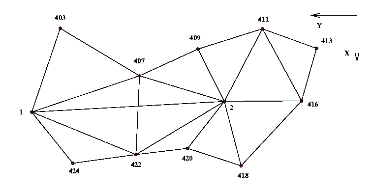
<?xml version="1.0" ?>

<gama-local xmlns="http://www.gnu.org/software/gama/gama-local">
<network axes-xy="sw">

<description>
XML input stream of points and observation data for the program GNU gama
</description>

<!-- parameters are expressed with empty-element tag -->

<parameters sigma-act = "aposteriori" />

<points-observations>

<!-- fixed point, constrained point -->

<point id="1" y="644498.590" x="1054980.484" fix="xy" />
<point id="2" y="643654.101" x="1054933.801" adj="XY" />

<!-- computed / adjusted points -->

<point id="403" adj="xy" />
<point id="407" adj="xy" />
<point id="409" adj="xy" />
<point id="411" adj="xy" />
<point id="413" adj="xy" />
<point id="416" adj="xy" />
<point id="418" adj="xy" />
<point id="420" adj="xy" />
<point id="422" adj="xy" />
<point id="424" adj="xy" />

<obs from="1">
     <direction  to=  "2" val=  "0.0000" stdev="10.0" />
     <direction  to="422" val= "28.2057" stdev="10.0" />
     <direction  to="424" val= "60.4906" stdev="10.0" />
     <direction  to="403" val="324.3662" stdev="10.0" />
     <direction  to="407" val="382.8182" stdev="10.0" />
     <distance   to=  "2" val= "845.777" stdev="5.0"  />
     <distance   to="422" val= "493.793" stdev="5.0"  />
     <distance   to="424" val= "288.301" stdev="5.0"  />
     <distance   to="403" val= "388.536" stdev="5.0"  />
     <distance   to="407" val= "498.750" stdev="5.0"  />
</obs>

<obs from="2">
     <direction  to=  "1" val="0.0000"   stdev="10.0" />
     <direction  to="407" val="22.2376"  stdev="10.0" />
     <direction  to="409" val="73.8984"  stdev="10.0" />
     <direction  to="411" val="134.2090" stdev="10.0" />
     <direction  to="416" val="203.0706" stdev="10.0" />
     <direction  to="418" val="287.2951" stdev="10.0" />
     <direction  to="420" val="345.6928" stdev="10.0" />
     <direction  to="422" val="368.9908" stdev="10.0" />
     <distance   to="407" val="388.562"  stdev="5.0"  />
     <distance   to="409" val="257.498"  stdev="5.0"  />
     <distance   to="411" val="360.282"  stdev="5.0"  />
     <distance   to="416" val="338.919"  stdev="5.0"  />
     <distance   to="418" val="292.094"  stdev="5.0"  />
     <distance   to="420" val="261.408"  stdev="5.0"  />
     <distance   to="422" val="452.249"  stdev="5.0"  />
</obs>

<obs from="403">
     <direction  to=  "1" val="0.0000"   stdev="10.0" />
     <direction  to="407" val="313.5542" stdev="10.0" />
     <distance   to="407" val="405.403"  stdev="5.0"  />
</obs>

<obs from="407">
     <direction  to=  "1" val="0.0000"   stdev="10.0" />
     <direction  to="403" val="55.1013"  stdev="10.0" />
     <direction  to="409" val="193.3410" stdev="10.0" />
     <direction  to=  "2" val="239.4204" stdev="10.0" />
     <direction  to="422" val="323.5443" stdev="10.0" />
     <distance   to="409" val="281.997"  stdev="5.0"  />
     <distance   to="422" val="346.415"  stdev="5.0"  />
</obs>

<obs from="409">
     <direction  to=  "2" val="0.0000"   stdev="10.0" />
     <direction  to="407" val="102.2575" stdev="10.0" />
     <direction  to="411" val="310.1751" stdev="10.0" />
     <distance   to="411" val="296.281"  stdev="5.0" />
</obs>

<obs from="411">
     <direction  to=  "2" val="0.0000"   stdev="10.0" />
     <direction  to="409" val="49.8647"  stdev="10.0" />
     <direction  to="413" val="291.4953" stdev="10.0" />
     <direction  to="416" val="337.6667" stdev="10.0" />
     <distance   to="413" val="252.266"  stdev="5.0"  />
     <distance   to="416" val="360.449"  stdev="5.0"  />
</obs>

<obs from="413">
     <direction  to="411" val="0.0000"   stdev="10.0" />
     <direction  to="416" val="295.3582" stdev="10.0" />
     <distance   to="416" val="239.745"  stdev="5.0"  />
</obs>

<obs from="416">
     <direction  to=  "2" val="0.0000"   stdev="10.0" />
     <direction  to="411" val="68.8065"  stdev="10.0" />
     <direction  to="413" val="117.9922" stdev="10.0" />
     <direction  to="418" val="348.1606" stdev="10.0" />
     <distance   to="418" val="389.397"  stdev="5.0"  />
</obs>

<obs from="418">
     <direction  to=  "2" val="0.0000"   stdev="10.0" />
     <direction  to="416" val="63.9347"  stdev="10.0" />
     <direction  to="420" val="336.3190" stdev="10.0" />
     <distance   to="420" val="246.594"  stdev="5.0"  />
</obs>

<obs from="420">
     <direction  to=  "2" val="0.0000"   stdev="10.0" />
     <direction  to="418" val="77.9221"  stdev="10.0" />
     <direction  to="422" val="250.1804" stdev="10.0" />
     <distance   to="422" val="228.207"  stdev="5.0"  />
</obs>

<obs from="422">
     <direction  to=  "2" val="0.0000"   stdev="10.0" />
     <direction  to="420" val="26.8834"  stdev="10.0" />
     <direction  to="424" val="225.7964" stdev="10.0" />
     <direction  to=  "1" val="259.2124" stdev="10.0" />
     <direction  to="407" val="337.3724" stdev="10.0" />
     <distance   to="424" val="279.405"  stdev="5.0"  />
</obs>

<obs from="424">
     <direction  to=  "1" val="0.0000"   stdev="10.0" />
     <direction  to="422" val="134.2955" stdev="10.0" />
</obs>

</points-observations>

</network>
</gama-local>
|
| [ < ] | [ > ] | [ << ] | [ Up ] | [ >> ] | [Top] | [Contents] | [Index] | [ ? ] |
gama-localYAML is a human-readable data-serialization language. It is commonly used for configuration files and in applications where data is being stored or transmitted. YAML targets many of the same communications applications as Extensible Markup Language but has a minimal syntax which intentionally differs from SGML. Wikipedia
In version 2.12 YAML support was added for gama-local as an
alternative to the existing XML input format. The YAML support is
limited only to conversion program gama-local-yaml2gkf but it
may be fully integrated in gama-local program later.
In GNU Gama YAML documents are based on four main nodes
   defaults:

   description:

   points:

   observations:
Where defaults and description are optional and
points and observations are mandatory and each can be
used only once. The order of the nodes is arbitrary.
Lets start with a full example
   defaults:
     sigma-apr : 5
     conf-pr:    0.95

   description: >-
     Example: a simple network

   points:
     - id:  1783
       y:   453500.000
       x:   104500.000
       adj: xy

     - id:  2044
       y:   461000.000
       x:   101000.000
       fix: xy

   observations:
     - from: 1783
       obs:
         - type:  direction
           to:    776
           val:   29.51661
           stdev: 2.0

         - type:  direction
           to:    351
           val:   94.22790
           stdev: 2.0

     - from: 351
       obs:
         - type:  direction
           to:    2044
           val:   170.48370
           stdev: 2.0

         - type:  distance
           to:    1783
           val:   5522.668
           stdev: 10.0

     - from: 462
       obs:
         - type:  direction
           to:    2505
           val:   299.99973
           stdev: 2.0
The description node is clearly the simplest one, it just
describes a simple text attached to the data. But still there may be a
catch. If the description contains colon (:), it might confuse
the YAML parser because it would be interpreted as a syntax
construction. To escape colon(s) in the description node we use
>- to prevent colons to be interpreted as a syntax
construction. Always using >- with description is a safe
bet.
The data structure of the YAML document is defined by indentation, this principle was inspired by Python programming language, where indentation is very important; Python uses indentation to indicate a block of code.
Practically all attribute names used in out YAML format are the same as in XML data format.
Lets have a look on some more examples. Within observations:
section we can define height differerence (another kind of a
measurement).
   observations:

     - height-differences:
         - dh:
             from: A
             to  : B
             val : 25.42
             dist: 18.1     # distance in km
         - dh:
             from: B
             to:   C
             val:  10.34
             dist:  9.4
Two remaining observation types are vectors and
coordinates.
   observations:
     - vectors:
       - vec:
           from: A
           to: S
           dx: 60.0070
           dy: 35.0053
           dz: 54.9953
       - vec:
           from: B
           to: S
           dx: -39.9974
           dy: 34.9928
           dz: 54.9976
and
   observations:
     - coordinates:
       - id: 403
         x: 1054612.59853
         y: 644373.60446
       - id: 407
         x: 1054821.17131
         y: 644025.97479

   ....

       - cov-mat:
           dim: 20
           band: 19
           upper-part:
             6.7589719e+01 1.8437742e+01 1.3176856e+01 ...
Typically any observation set can define its covariance matrix.
You may wish to compare YAML and XML data files available from Gama tests suite in tests/gama-local/input directory (files *.gkf and *.yaml).
The gama-local input xml data can be formally validated against the XSD
definition. Unfortunatelly there is no formal definition of YAML
input. Within the testing suite of GNU Gama project we have a test
that validates all available YAML files converted to XML by the formal
XSD definition, see the test xmllint-gama-local-yaml2gkf.
| 3.1 YAML support |
| [ < ] | [ > ] | [ << ] | [ Up ] | [ >> ] | [Top] | [Contents] | [Index] | [ ? ] |
GNU Gama YAML input format is dependent on C++ YAML-CPP library written by Jesse Beder https://yaml.org/. With the Gama primary build system (autotools) you need to install the library at your system, for example on Debian like systems it is libyaml-cpp-dev package.
A different solution is used in the alternative Gama cmake based
build, where the source codes are expected to be available from the
lib directory. Change to "GNU Gama sources"/lib and clone the
git repository.
   cd "GNU Gama sources"/lib
   git clone https://github.com/jbeder/yaml-cpp
| [ < ] | [ > ] | [ << ] | [ Up ] | [ >> ] | [Top] | [Contents] | [Index] | [ ? ] |
gama-localThe input data for a local geodetic network adjustment (program
gama-local) can be strored in SQLite 3 database file.
The general information about SQLite can be found at
Input data (points, observations and other related information) are stored in SQLite database file. Native SQLite C/C++ API is used for reading SQLite database file. It is described at
http://www.sqlite.org/c3ref/intro.html
Please note if you compile GNU Gama as described in Install and SQLite library is not installed on your system, GNU Gama would be compiled without SQLite support.
SQL schema (CREATE statements) is in gama-local-schema.sql file
which is part of GNU Gama distribution and is in the xml directory.
All tables for gama-local are prefixed with gnu_gama_local_.
In the documentation table names are referred without this prefix.
For example table gnu_gama_local_points is referred as points.
Database scheme used for SQLite database is also valid in other SQL database systems. Almost every column has some constraint to ensure correctness.
You can convert existing XML input file to SQL commands with
program gama-local-xml2sql, for example
$ gama-local-xml2sql geodet-pc geodet-pc-123.gkf geodet-pc.sql |
| 4.1 Working with SQLite database | ||
| 4.2 Units in SQL tables | Units of values in SQL tables | |
| 4.3 Network SQL definition | Tables configurations and description
| |
4.4 Table points | ||
4.5 Table clusters | ||
4.6 Table covmat | ||
4.7 Table obs | ||
4.8 Table coordinates | ||
4.9 Table vectors | ||
| 4.10 Example of local geodetic network in SQL | Obtaining example of local geodetic network in SQL |
| [ < ] | [ > ] | [ << ] | [ Up ] | [ >> ] | [Top] | [Contents] | [Index] | [ ? ] |
First of all you have to create tables for GNU Gama in SQLite database file
(here with db extension, but you can choose your own, e.g. sqlite).
$ sqlite3 gama.db < gama-local-schema.sql |
You can check created tables by following commands (fist in command line, second in SQLite command line).
$ sqlite3 gama.db sqlite> .tables |
Output should look like this:
gnu_gama_local_clusters gnu_gama_local_descriptions gnu_gama_local_configurations gnu_gama_local_obs gnu_gama_local_coordinates gnu_gama_local_points gnu_gama_local_covmat gnu_gama_local_vectors |
When you have created tables you can import data. One way is to process file with SQL statements.
$ sqlite3 gama.db < geodet-pc.sql |
Another way can be filing database file in another program.
For using sqlite3 command you need a command line
interface for SQLite 3 installed on your system (e.g. sqlite3 package).
| [ < ] | [ > ] | [ << ] | [ Up ] | [ >> ] | [Top] | [Contents] | [Index] | [ ? ] |
In the gama-local SQLite database, distances are given in meters
and their standard deviations (rms errors) in millimeters.
Angular values are given in radians as well as their standard deviations.
Conversions between radians, gons and degrees:
    rad = gon * pi / 200
    rad = deg * pi / 180
    gon = rad * 200 / pi
    deg = rad * 180 / pi
|
| [ < ] | [ > ] | [ << ] | [ Up ] | [ >> ] | [Top] | [Contents] | [Index] | [ ? ] |
Network definitions are stored in the configurations table.
This table contains all parameters for each network such as value of a
priori reference standard deviation or orientation of the xy
orthogonal coordinate system axes.
It is obvious that in one database file can be stored more networks (configurations).
Configuration descriptions (annotation or comments) are stored separately
in table descriptions.
The description is split to many records because of compatibility with various
databases (not all databases implements type TEXT).
Field (attribute) conf_id identifies a configuration in the database.
Field conf_name is used to identify configuration outside the database
(e.g. parameter in command-line when reading data from database
to gama-local).
Table configurations contains all parameters specified in
tag <parameters /> (see section Network parameters) and also
gama-local command line parameters (see section Program gama-local).
The list of all table attributes (parameters) follows.
sigma_apr value of a priori reference standard deviation—square
root of reference variance (default value 10)
conf_pr confidence probability used in statistical tests
(dafault value 0.95)
tol_abs tolerance for identification of gross
absolute terms in project equations (default value 1000 mm)
sigma_act actual type of reference standard deviation
use in statistical tests (aposteriori | apriori); default value
is aposteriori
update_cc enables user to control
if coordinates of constrained points are updated in iterative
adjustment. If test on linerarization fails (see section Test on linearization),
Gama tries to improve approximate coordinates of adjusted points and
repeats the whole adjustment. Coordinates of constrained points are
implicitly not changed during iterations.
Acceptable values are yes, no, default value
is yes.
axes_xy
orientation of axes x and y; value
ne implies that axis x is oriented north and axis y
is oriented east. Acceptable values are ne, sw,
es, wn for left-handed coordinate systems and en,
nw, se, ws for right-handed coordinate systems
(default value is ne).
angles right-handed defines counterclockwise observed angles
and/or directions, value left-handed defines clockwise observed
angles and/or directions (default value is left-handed).
epoch
is measurement epoch.
It is floating point number
(default value is 0.0).
algorithm
specifies numerical method used for solution of the adjustment.
For Singular Value Decomposition set value to svd.
Value gso stands for block matrix algorithm GSO by Frantisek Charamza
based on Gram-Schmidt orthogonalization,
value cholesky for Cholesky decomposition of semidefinite matrix
of normal equations
and value envelope for a Cholesky decomposition with
envelope reduction of the sparse matrix.
Default value is svd.
ang_units
Angular units of angles in gama-local output.
Value 400 stands for gons and value 360 for degrees
(default value is 400).
Note that this doesn’t effect units of angles in database.
For further information about angular units see Angular units.
latitude
is mean latitude in network area.
Default value is 50 (gons).
ellipsoid
is name of ellipsoid (see section Supported ellipsoids).
All fields are mandatory except ellipsoid field.
For additional information about handling geodetic systems in gama-local
see Tags <gama-local> and <network>.
Example (configuration table contents):
conf_id|conf_name|sigma_apr|conf_pr|tol_abs|sigma_act |update_cc|... --------------------------------------------------------------------- 1 |geodet-pc|10.0 |0.95 |1000.0 |aposteriori|no |... ... axes_xy|angles |epoch|algorithm|ang_units|latitude|ellipsoid --------------------------------------------------------------------- ... ne |left-handed|0.0 |svd |400 |50.0 | |
The list of description table attributes follows.
conf_id
is id of configuration which description (text) belongs to.
id
identifies text in a database.
text
is part of configuration description.
Its SQL type is VARCHAR(1000).
There can be more than one text for one configuration. All texts related to one configuration are concatenated to one description.
Example (description table contents):
conf_id|indx|text ----------------------------------------------- 1 |1 |Frantisek Charamza: GEODET/PC, ... |
| [ < ] | [ > ] | [ << ] | [ Up ] | [ >> ] | [Top] | [Contents] | [Index] | [ ? ] |
pointsconf_id
is id of configuration which points belongs to.
id
identifies point in a database and also in an output.
It is mandatory and it is character string (SQL type is VARCHAR(80)).
Point id has to be unique within one configuration.
In documentation it is referred as point identification or point id.
x, y and z
coordinates of a point.
Coordinate z is considered as height.
txy and tz
specify the type of coordinates x, y and z.
Acceptable values are fixed, adjusted and constrained
(there is no default value).
For details see Points.
Example (table contents):
conf_id|id |x |y |z|txy |tz ------------------------------------------ 1 |201|78594.91|9498.26| |fixed | 1 |205|78907.88|7206.65| |fixed | 1 |206|76701.57|6633.27| |fixed | 1 |207| | | |adjusted| |
| [ < ] | [ > ] | [ << ] | [ Up ] | [ >> ] | [Top] | [Contents] | [Index] | [ ? ] |
clustersThe cluster is a group of observations with the common covariance matrix. The covariance matrix allows to express any combination of correlations among observations in cluster (including uncorrelated observations, where covariance matrix is diagonal). For explanation see Observation data and points.
In the database observations are stored in three tables:
obs, coordinates and vectors.
Cluster’s covariance matrix is stored in table covmat.
Every observation, vector or coordinate in database has to be in some cluster.
conf_id
is id of configuration which cluster belongs to.
ccluster
identifies a cluster within one configuration.
dim and band
specify dimension and bandwidth of covariance matrix.
The bandwidth of the diagonal matrix is equal to 0 and a
fully-populated covariance matrix has a bandwidth of dim-1
(band maximum possible value is dim-1).
tag
specifies type of observations in cluster which also implies the table
where they are stored in.
obs and height-differences stand for obs table,
coordinates and vectors stand for coordinates table
and vectors table respectively.
Observations, vectors and coordinates are identified by
configuration id (conf_id), cluster id ccluster
and theirs index (indx).
Observation index (indx) has to be unique within observations
of one cluster (which belongs to one configuration).
The same applies for vectors and coordinates.
See also Set of observations.
Example (table contents):
conf_id|ccluster|dim|band|tag ----------------------------- 1 |1 |3 |0 |obs 1 |4 |4 |0 |obs |
| [ < ] | [ > ] | [ << ] | [ Up ] | [ >> ] | [Top] | [Contents] | [Index] | [ ? ] |
covmatValues of cluster covariance matrix are stored
in covmat table.
Attributes conf_id, ccluster identifies covariance matrix.
Value position in matrix is specified by rind and cind fields.
conf_id
is id of configuration which cluster belongs to.
ccluster
is id of cluster which matrix belongs to.
rind
is row number in covariance matrix
cind
is column number covariance matrix
val
is value itself (variance or covariance).
Values rind and cind have to respect dim and band
specified in table clusters.
If value in covariance matrix is not specified (record is missing),
it is considered to be zero.
Example (table contents):
conf_id|ccluster|rind|cind|val -------------------------------- 1 |1 |1 |1 |400.0 1 |1 |2 |2 |400.0 1 |1 |3 |3 |400.0 1 |4 |1 |1 |400.0 1 |4 |2 |2 |400.0 1 |4 |3 |3 |400.0 1 |4 |4 |4 |400.0 |
| [ < ] | [ > ] | [ << ] | [ Up ] | [ >> ] | [Top] | [Contents] | [Index] | [ ? ] |
obsTable obs contains simple observations like direction or distance.
conf_id
is id of configuration which cluster belongs to.
ccluster
is id of cluster which observation belongs to.
indx
identifies observation within cluster.
It has to be positive integer.
tag
specifies a type of an observation.
Allowed tags follows.
direction
for directions.
distance
for horizontal distances.
angle
for angles.
s-distance
for slope distances (space distances).
z-angle
for zenith angles.
azimuth
for azimuth angles.
dh
for leveling height differences.
from_id
is stand point identification.
It is mandatory and it must not differ within one cluster for observations
with tag = 'direction' .
to_id
is target identification (mandatory).
to_id2
is second target identification.
It is valid and mandatory only for angles (tag = 'angle').
val
is observation value.
It is mandatory for all observation types.
stdev
is value of standard deviation.
It is used when variance in covariance matrix is not specified.
from_dh
is value of instrument height (optional).
to_dh
is value of reflector/target height (optional).
to_dh2
is value of second reflector/target height (optional).
It is valid only for angles.
dist
is distance of leveling section. It is valid only for height-differences (tag = 'dh').
rejected
specifies whether observation is rejected (passive) or not.
Value 0 stand for not rejected, value 1 for rejected.
It is mandatory. Default value is 0.
Example (table contents without empty columns):
conf_id|ccluster|indx|tag |from_id|to_id|val |rejected --------------------------------------------------------------------- 1 |1 |1 |direction|201 |202 |0.0 |0 1 |1 |2 |direction|201 |207 |0.817750284544|0 1 |1 |3 |direction|201 |205 |2.020073921388|0 |
| [ < ] | [ > ] | [ << ] | [ Up ] | [ >> ] | [Top] | [Contents] | [Index] | [ ? ] |
coordinatesTable coordinates contains control (known) coordinates.
conf_id
is id of configuration which cluster belongs to.
ccluster
is id of cluster which coordinates belongs to.
indx
identifies coordinates within cluster.
It has to be positive integer.
id
is point identification.
x,
y
and
z
are coordinates.
rejected specifies whether observation is rejected (passive) or not.
Value 0 stand for not rejected, value 1 for rejected.
Default value is 0.
See also Control coordinates.
| [ < ] | [ > ] | [ << ] | [ Up ] | [ >> ] | [Top] | [Contents] | [Index] | [ ? ] |
vectorsTable vectors contains coordinate differences (vectors).
conf_id
is id of configuration which cluster belongs to.
ccluster
is id of cluster which vector belongs to.
indx
identifies vector within cluster.
It has to be positive integer.
from_id
is point identification.
It identifies initial point.
to_id
is point identification.
It identifies terminal point.
dx,
dy
and
dz
are coordinate differences.
from_dh
is value of initial point height.
It is optional.
to_dh
is value of terminal point height.
It is optional.
rejected integer default 0 not null,
See also Coordinate differences (vectors).
| [ < ] | [ > ] | [ << ] | [ Up ] | [ >> ] | [Top] | [Contents] | [Index] | [ ? ] |
Providing complete example would be reasonable because of its extent. However, you can obtain example by following these instructions:
Create a file with XML representation of network by copy and paste example
from Example of local geodetic network to a new file.
Note that file should start with <?xml version="1.0" ?> (no whitespace).
Alternatively you can use existing XML file from collection of sample networks
(see Download).
Then you can convert your XML file (here example_network.xml)
to SQL statements by program gama-local-xml2sql
(the path depends on your Gama installation).
$ gama-local-xml2sql example_net example_network.xml example_network.sql |
Now you have example network (configuration example_net)
in the form of SQL INSERT statements
in the file example_network.sql.
Another representations you can create and fill SQLite database (for details see Working with SQLite database):
$ sqlite3 examples.db < gama-local-schema.sql $ sqlite3 examples.db < example_network.sql $ sqlite3 examples.db |
Once you have SQLite database, you can work with it from SQLite command line. You can get nice output by executing following commands.
sqlite> .mode column sqlite> .nullvalue NULL sqlite> SELECT * FROM gnu_gama_local_configurations; sqlite> SELECT * FROM gnu_gama_local_points; sqlite> SELECT * FROM gnu_gama_local_clusters; sqlite> SELECT * FROM gnu_gama_local_covmat; sqlite> SELECT * FROM gnu_gama_local_obs; |
Or you can get database dump (CREATE and INSERT statements) by
sqlite> .dump |
If it is not enough for you, you can try one of GUI tools for SQLite.
| [ < ] | [ > ] | [ << ] | [ Up ] | [ >> ] | [Top] | [Contents] | [Index] | [ ? ] |
gama-localAdjustment of local geodetic network is a classical case of adjustment of indirect observations. After estimation of approximate values of unknown parameters (coordinates of points) and linearization of functions describing relations between observations and parameters we solve linear system of equations
(1) Ax = b + v, |
where A is coefficient matrix, b is vector of absolute terms
(right hand side) and v is vector of residuals.
This system is (generally) overdetermined and we seek
the solution x satisfying the basic criterion of Least Squares
(2) v'Pv = min, |
where P is weight matrix. This criterion unambiguously defines the
shape of adjusted network.
Geodetic adjustment is traditionally computed as the solution of normal equations (2)
(a) Nx = n, where N=A'PA and n=A'Pb. |
In the case of free network, i.e. network with no fixed
coordinates (or network without sufficient number of fixed
coordinates), the system (1) is singular, matrix A has linearly
dependent columns, and there is infinite number of solutions x.
To define a unique solution x we need to definine a set of
constriant equations (inner constraints)
(b) Cx = c |
to minimize
(c) v'Pv - 2k'(Cx - c) = min |
where r is the vector of residuals, r = Ax - b, k is a
vector of so called Lagrange multipliers and adjusted vector x
is obtained from solution of
(d)      ( A'PA, C') (x) = (A'Pb)
         ( C,    0 ) (k) = (  c )
|
In gama-local a slightly different approach is used, we define
a second regularization criterion as
(3) \sum x_i^2 = min, for all selected i |
stating that at the same time with (2) we demand that the sum of squares corrections of selected parameters is minimal (corrections of unknown parameters with indexes from the set of all selected unknowns. Geometrically this criterion is equivalent to adjustment of the network according to (2) with simultaneous transformation to the selected set of fiducial points. This transformation does not change the shape of adjusted network.
Often it is advantageous to work with a homogenized system, ie. with the system of project equations in which coefficient of each row and absolute term are multiplied by square root of the weight of corresponding observation.
(4) ~A x = ~b, |
where ~A = P^1/2 A, ~b = P^1/2 A. Symbol P^1/2 denotes diagonal matrix of square roots of observation weights (or Cholesky decomposition of covariance matrix in the case of correlated observations). To criterion (2) corresponds in the case of homogenized system criterion
(5) ~v'~v = min. |
Normal equations are clearly equivalent for both systems.
| [ < ] | [ > ] | [ << ] | [ Up ] | [ >> ] | [Top] | [Contents] | [Index] | [ ? ] |
For computation of coefficients in system (1) (ie. during linearization) we need, first of all, an estimate of approximate coordinates of points and approximate values of orientations of observed directions sets.
Approximate values of unknown parameters are usually not known and we
have to compute them from the available observations. For approximate
value of orientation program gama-local uses median of all estimates
from the given set of directions to the points with known coordinates.
Median is less sensitive to outliers than arithmetic mean which is
normally used for approximate estimate of orientations
During the phase of computation of approximate coordinate of points,
program gama-local walks through the list of computed points
and for each point gathers all determining elements pointing to
points with known or previously computed coordinates.
Determining elements are
distance between given and computed points
For all combinations of determining elements program gama-local
computes intersections and estimates approximate coordinates as the
median of all available solutions.
If at least one point was resolved while iterating through the list, the whole cycle is repeated.
If no more coordinates can be solved using intersections and points with unknown coordinates are remaining, program tries to compute coordinates of unresolved points in a local coordinates system and obtain their coordinates using similarity transformation. If a transformation succeeds to resolve coordinates at least one computed point and there are still some points without coordinates left, the whole process is repeated. Classes for computation of approximate coordinates have been written by Jiri Vesely.
If program gama-local fails to compute approximate coordinates
of some of the network points, they are eliminated from the
adjustment and they are listed in the output listing.
With the outlined strategy, program gama-local is able to estimate
approximate coordinates in most of the cases we normally meet in
surveying profession. Still there are cases in which the solution fails.
One example is an inserted horizontal traverse with sets of observed
direction on both ends but without a connecting observed distance. The
solution of approximate coordinates can fail when there is a number of
gross error for example resulting from confusion of point
identifications but in normal situations, leaving computation of
approximate coordinates on program gama-local is recommended.
Computation of approximate coordinates of points ************************************************ Number of points with given coordinates: 2 Number of solved points : 2 Number of observations : 4 ----------------------------------------------------- Successfully solved points : 0 Remaining unsolved points : 2 List of unresolved points ************************* 422 424 |
| [ < ] | [ > ] | [ << ] | [ Up ] | [ >> ] | [Top] | [Contents] | [Index] | [ ? ] |
One of parameters in XML input of program gama-local is tolerance
tol-abs for detecting of gross absolute terms in
project equations. Observations with outlying absolute terms
are always excluded from adjustment.
For measured distances program tests difference between observed value d_i and distance computed from approximate coordinates d_0
|d_i - d_0| > |
for observed directions program gama-local tests transverse deviation
corresponding to absolute term b_i from
project equations (1)
| b_i | d_0 > |
and similarly for angles, program tests the greater of two deviations corresponding to left and right distances (left and right arm of the angle)
|b_i| max{ d_{0_l}, d_{0_r} } > |
Default value of parameter tol-abs is 1000 mm.
Outlying absolute terms in project equations ******************************************** i standpoint target observed absolute =========================================== value ===== term == 2 103 104 dir. 301.087900 -9989.1 Observations with outlying absolute terms removed |
| [ < ] | [ > ] | [ << ] | [ Up ] | [ >> ] | [Top] | [Contents] | [Index] | [ ? ] |
Program gama-local uses two basic statistical parameters
conf-pr) and
sigma-act).
Confidence probability determines significance level on which statistical tests of adjusted quantities are carried. Actual type of reference standard deviation m0_a specifies whether during statistical analysis we use an a priori reference standard deviation m0 or an a posteriori estimate m0’. On the type of actual reference standard deviation depends the choice of density functions of stochastic quantities in statistical analysis of the adjustment.
The standard deviantion of an adjusted quantity is computed in dependence of the choice of actual type of reference standard deviation m0_a according to formula
m0_a sqrt(q)
where q is the weight coefficient of the corresponding adjusted
unknown parameter or observation. Apart from the standard deviation,
program gama-local computes for the adjusted quantity its
confidence interval in which its real value is located
with the probabilityP.
| [ < ] | [ > ] | [ << ] | [ Up ] | [ >> ] | [Top] | [Contents] | [Index] | [ ? ] |
Null hypothesis H_0: m0 = m0’ is tested versus alternative hypothesis H_1: m0 neq m0’. Test criterion is ratio of a posteriori estimate of reference standard deviation
m0' = sqrt( v'P v / r). |
and a priori reference standard deviation m0 (input data parameter
m0-apr). For given significance level alpha lower and
upper bounds of interval (L, U) are computed so, that if
hypothesis H_0 is true, probabilities P(m0’/m0
le D) and P(m0’/m0 ge H) are equal to
alpha/2. Lower and upper bounds of the interval are computed as
         L = sqrt((Chi^2_{1-alpha/2,r})/r),
         U = sqrt((Chi^2_{ alpha/2 ,r})/r).
|
Probability
P(L < m0'/m0 < U) = |
is by default 95%, this corresponds to 5% confidence level test.
Exceeding the upper limit H of the confidence interval can be caused even by a single gross error (one outlying observation). Method of Least Squares is generally very sensitive to presence of outliers. Safely can be detected only one observation whose elimination leads to maximal decrease of a posteriori estimate of reference standard deviation
(6)      m0''  = sqrt{(v'P v - delta)/(r-1)},
         delta = max(v_i^2/q_vi),
|
where
(7) q_vi = 1/p_i - q_Li |
is weight coefficient of i-th residual. If the set of observations contains only one gross error, the outlying observation is likely to be detected, but this can not be guaranteed.
In addition, program gama-local computes a posteriori estimate
of reference standard deviation separately for horizontal distances
and directions and/or angles after formula from
m0'_t = sqrt(sum{~v^2_it}) / sum{~q_vi}), t=d,s,
|
where symbol t denotes observed distances, directions and/or angles.
m0 apriori : 10.00 m0' empirical: 9.64 [pvv] : 3.43560e+03 During statistical analysis we work - with empirical standard deviation 9.64 - with confidence level 95 % Ratio m0' empirical / m0 apriori: 0.964 95 % interval (0.773, 1.227) contains value m0'/m0 m0'/m0 (distances): 0.997 m0'/m0 (directions): 0.943 Maximal decrease of m0''/m0 on elimination of one observation: 0.892 Maximal studentized residual 2.48 exceeds critical value 1.95 on significance level 5 % for observation #35 <distance from="407" to="422" val="346.415" stdev="5.0" /> |
| [ < ] | [ > ] | [ << ] | [ Up ] | [ >> ] | [Top] | [Contents] | [Index] | [ ? ] |
Program gama-local lists separately review of coordinates of fixed and
adjusted points; adjusted constrained coordinates are marked with
*; see equation (3). Adjusted coordinate standard deviations
m_x and m_y, and values for computing confidence intervals
are given in the listing of adjusted coordinates (Parameters of statistical analysis). In the review index i is the index of unknown
x_i from the system of project equations (1) corresponding to the
point coordinates x and y.
Fixed points
************

       point         x              y
========================================

           1  1054980.484     644498.590
           2  1054933.801     643654.101


Adjusted coordinates
********************

  i        point    approximate  correction  adjusted    std.dev conf.i.
====================== value ====== [m] ====== value ========== [mm] ===

             422
  2            x   1055167.22747  -0.00510 1055167.22237     2.7     5.4
  3            y    644041.46119   0.00023  644041.46142     2.5     5.1

             424
  4            X * 1055205.41198  -0.00056 1055205.41142     3.1     6.3
  5            Y *  644318.24425  -0.00125  644318.24300     3.6     7.2
|
For adjusted points, program summarizes information on standard ellipses, confidence ellipses, mean square positional errors (m_p), mean coordinate errors (m_xy) and coefficients g characterizing position of approximate coordinates with regard to the confidence ellipse.
Mean errors and parameters of error ellipses
********************************************

  point     mp      mxy      mean error ellipse  conf.err. ellipse   g
========== [mm] == [mm] ==== a [mm] b  alpha[g] ==== a' [mm] b' ========

    422     3.6     2.6     2.7     2.5   187.0     6.8     6.4     0.8
    424     4.7     3.4     3.7     2.9   131.8     9.5     7.4     0.2
    403     5.7     4.0     4.3     3.6    78.9    11.0     9.3     1.1
|
Mean square positional error m_p and mean coordinate error (m_xy) are computed as
m_p = sqrt(m_y^2 + m_x^2), m_xy = m_p / sqrt(2), |
where m_y^2 and m_x^2 are squares of standard deviations (variances) of adjusted points coordinates.
Semimajor and semiminor axes of standard ellipse are denoted as a and b in the listing, bearing of semimajor axis is denoted as alpha and they are computed from covariances of adjusted coordinates
         a = sqrt(1/2(cov_yy + cov_xx + c),
         b = sqrt(1/2(cov_yy + cov_xx - c),

         c = sqrt( (cov_xx - cov_yy)^2 + 4(cov_xy)^2 ),

         tan 2alpha = 2(cov_xy) / (cov_xx - cov_yy).
|
The angle alpha (the bearing of semimajor axis) is measured clockwise from X axis.
Probability that standard ellipse covers real position of a point is
relatively low. For this reason program gama-local computes extra
confidence ellipse for which the probability of covering real
point position is equal to the given confidence probability. Both
ellipses are located in the same center, they share the same bearing of
semimajor axes and they are similar. For lengths of their semi-axis
holds
a' = k_p a, b' = k_p b, |
where k_p is a coefficient computed for the given probability P as defined in Parameters of statistical analysis.
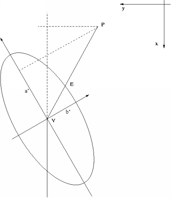
Position of approximate coordinates of an adjusted point with respect to its confidence ellipse are expressed by a coeeficient g Three cases are possible
The coefficient g is calculated from formula
g = sqrt( (a_0 / a')^2 + (b_0/b')^2 ) |
where
         b_0 = delta_y cos(alpha) - delta_x sin(alpha),
         a_0 = delta_y sin(alpha) - delta_x cos(alpha)
|
symbol delta is used for correction of approximate coordinates and alpha is bearing of confidence ellipse semimajor axis.
If network contains sets of observed directions, program writes information on corresponding adjusted orientations, standard deviations and confidence intervals. Index i is the same as in the case of adjusted coordinates the index of i-th adjusted unknown in the project equations.
Adjusted bearings ***************** i standpoint approximate correction adjusted std.dev conf.i. ==================== value [g] ==== [g] === value [g] ======= [cc] === 1 1 296.484371 -0.000917 296.483454 5.1 10.3 10 2 96.484371 0.000708 96.485079 5.1 10.4 21 403 20.850571 -0.001953 20.848618 8.8 17.7 |
| [ < ] | [ > ] | [ << ] | [ Up ] | [ >> ] | [Top] | [Contents] | [Index] | [ ? ] |
In the review of adjusted observations program gama-local prints index of
the observation, index of the row in matrix A in the system (1),
identifications of standpoint and target point, type of the observation,
its approximate and adjusted value, standard deviation and confidence
interval.
Adjusted observations ********************* i standpoint target observed adjusted std.dev conf.i. ===================================== value ==== [m|g] ====== [mm|cc] == 1 1 2 dis. 845.77700 845.77907 3.0 6.1 2 422 dir. 28.205700 28.205613 5.1 10.3 3 424 dir. 60.490600 60.491359 6.7 13.6 |
Review of residuals serves for analysis of observations and containts
values of normalized or studentized residuals (depending on type of
m0_a used) and three characteristics.
Theese are coefficient f identifying weak network elements and
estimates of real error of observation e-obs and real error of
its adjusted value e-adj, see definition in the following text.
If normalized or studentized residual exceeds critical value for the
given confidence probability, it is marked in the review with symbol
c (critical) and maximal normalized or studentized residual is
marked with symbol m.
Residuals and analysis of observations ************************************** i standpoint target f[%] v |v'| e-obs. e-adj. ======================================== [mm|cc] =========== [mm|cc] === 1 1 2 dir. 47.4 9.170 1.1 12.7 3.5 2 422 dir. 47.0 -0.873 0.1 -1.2 -0.3 3 424 dir. 30.3 7.588 1.1 14.8 7.2 |
| [ < ] | [ > ] | [ << ] | [ Up ] | [ >> ] | [Top] | [Contents] | [Index] | [ ? ] |
When planning observations in a geodetic network we always try to guarantee that all observed elements are checked by other measurements. Only with redundant measurements it is possible to adjust observations and possibly remove blunders that might otherwise totaly corrupt the whole set of measurements. Apart from sufficient number of redundant observations the degree of control of single observed elements is given by the network configuration, ie. its geometry.
Less controlled observations represent weak network elements and they can in extreme cases even disable detection of gross observational errors as it is in the case of uncontrolled observations. There are two limit cases of observation control
Weakly controlled or uncontrolled observations can result even from elimination of certain suspisios observations during analysis of adjusment.
Standard deviation of adjusted observations is less than standard deviation of the measurement. Degree of observation control in network is defined as coefficient
(8) f = 100 (m_l - m_L)/m_l, |
where m_l is standard deviation of observed quantity and m_L is standard deviation computed from a posteriori reference standard deviation m0. We consider observed network element to be
u),
w).
| [ < ] | [ > ] | [ << ] | [ Up ] | [ >> ] | [Top] | [Contents] | [Index] | [ ? ] |
Acording to previous section we can consider an observation to be controlled if its coefficient f > 0.1. Any controlled observation can be eliminated from the network without corrupting the network consistency—network reduced by one controlled observation can be adjusted and all unknown parameters can be compute without the eliminated observation.
Estimate of real error of i-th observation is defined as
(9) e_li = L^red_i - l_i, |
where e_li is value of i-th observation and is value of i-th network element computed from adjusted coordinates and/or orientations of the reduced network. Similarly is defined the estimate of real error of a residual
(10) e_vi = L^red_i - L_l. |
Adjustment results are the best statistical estimate of unknown parameters that we have. This holds true even for adjustment of reduced network which is not influenced by real error of i-th observation. On favourable occasions differences (9) and (10) can help to detect blunders but to interpret these estimates as real errors is possible only with substantial exaggeration. These estimates fail when there are more than one significant observational error. Generally holds tha the weaker the element is controlled in netowrk the less reliable these estimates are.
Estimate of real error of an observation computes program gama-local as
e_li = v_i/(p_i q_vi) |
and estimate of real error of a residual as
e_vi = e_li - v_i. |
| [ < ] | [ > ] | [ << ] | [ Up ] | [ >> ] | [Top] | [Contents] | [Index] | [ ? ] |
Mathematical model of geodetic network adjustment in gama-local
is defined as a set of known real-valued differentiable functions
(11) L^* = f(X^*) |
where
L^*
is a vector of theoretical correct observations and
X^*
is a vector of correct values of parameters. For the given sample set
of observations L and the unknown vector of residuals v we
can express the estimate of parameters X as a nonlinear set of
equations
(12) L + v = f(X). |
With approximate values X_0 of unknown parameters
(12) X = X_0 + x |
we can linearize the equations (12)
L + v = f(X_0) + f'(X_0)x. |
yielding the linear set of equations (1)
Unknown parameters in gama-local mathematical model are points
coordinates and orientation angles (transforming observed directions
to bearings). The observables described by functions (12) belong into
two classes
Internally in gama-local unknown corrections to linear
observables are computed in millimeters and corrections to angular
observables in centigrade seconds. To reflect the internal units in
used all partial derivatives of angular observables by coordinates are
scaled by factor
2000/pi.
When computing coefficients of project equations (1) we expect that approximate coordinates of points are known with sufficient accuracy needed for linearization of generally nonlinear relations between observations and unknown paramters. Most often this is true but not always and generally we have to check how close our approximation is to adjusted parameters.
Generally we check linearization in adjustment by double calculation of residuals
         v^I  = Ax - b,
         v^II = ~l(~x) - l,
|
Program gama-local similarly computes and tests differences in
values of adjusted observations once computed from residuals
and once from adjusted coordinates. For measured directions
and angles gama-local computes in addition transverse deviation
corresponding to computed angle difference in the distance
of target point (or the farther of two targets for angle).
As a criterion of bad linearization is supposed positional
deviation greater or equal to 0.0005 millimetres.
Test of linearization error *************************** Diffs in adj. obs from residuals and from adjusted coordinates ************************************************************** i standpoint target observed r difference ================================= value = [mm|cc] = [cc] == [mm]= 2 3022184030 3022724008 dist. 28.39200 -7.070 -0.003 3 3022724002 dist. 72.30700 -18.815 -0.001 7 3000001063 dir. 286.305200 11.272 -0.002 -0.001 8 3022724008 dir. 357.800600 -23.947 0.037 0.002 |
From the practical point of view it might seem that the tolerance
0.0005 mm for detecting poor linearization is too strict. Its
exceeding in program gama-local results in repeated adjustment
with substitute adjusted coordinates for approximate. Given tolerance
was chosen so strict to guarantee that listed output results would
never be influenced by linearization and could serve for verification
and testing of numerical solutions produced by other programs.
Iterated adjustement with successive improvement of approximate unknown coordinates converges usually even for gross errors in initial estimates of unknown coordinates. If the influence of linearization is detected after adjustment, typically only one iteration is sufficient for recovering.
For any automatically controlled iteration we have to set up certain
stopping criterion independent on the convergence and results obtained.
Program gama-local computes iterated adjustment three times at maximum.
If the bad linearization is detected even after three readjustments it
signals that given network configuration is somehow suspicious.
| [ < ] | [ > ] | [ << ] | [ Up ] | [ >> ] | [Top] | [Contents] | [Index] | [ ? ] |
Symbols and names used in adjustment statistics.
| Symbol | Description |
|---|---|
| v, V | residual, vector of residuals |
| p, P | observation weight, matrix of weights |
| [pvv] | sum of weighted residuals v’Pv.
The summation symbol [.] used to be popular in geodetic literiture, namely in connection with description of normal equations, during pre-computer era. It was introduced by Carl Friedrich Gauss who also introduce symbol P for weights (Latin pondus means weight). Letter V for adjustment reductions comes from German Verbesserung. We use [pvv] symbol only in html and text adjustment output. Sic transit gloria mundi. |
| Ax = b, P | design matrix, right-hand side (rhs) and weight matrix P |
| r | redundancy, typically number of columns minus rows of A |
| Nx = n | normal equations,
N = A’PA,
n = A’Pb.
The method of least squares can be solved directly from Ax=b. which is generally a more numerically stable solution |
| Q = inv(N) | cofactor matrix for adjusted unknowns (matrix of weight coefficients, cofactors, of adjusted unknowns) |
| Q_L = AQA’ | cofactor matrix for adjusted observations |
| f[%] | degree of control of an observation in the network, spans from 0% (uncontrolled, e.g. observed direction and distance to an isolated adjustment point) to 100% (fully controled, e.g. measured distance between two fixed points) |
| m0 | a priori reference standard deviation. |
| m0’ | a posteriori estimate of reference standard deviation |
| m0” | minimal a posteriori estimate of reference standard deviation after removal one observation (removal of the observation leading to minimal value of m0”) |
| g | position of approximate coordinates xy of the adjusted point with
respect to its confidence ellipse (g < 1 approximate coordinates
are located inside the ellipse; g = 1 on the ellipse; g > 1
outside the ellipse). Zero value of g indicates that approximate and adjusted coordinates are identical. This situation typically happens when iterative adjustement is needed due to poor initial linearization (initial approximate coordinates are too far from the adjusted) and the iterative process ends up with identical approximate and adjusted coordinates. |
| [ < ] | [ > ] | [ << ] | [ Up ] | [ >> ] | [Top] | [Contents] | [Index] | [ ? ] |
| 6.1 Observation data and points | ||
| 6.2 Supported ellipsoids | ||
| 6.3 Transformation from spatial to geographical coordinates | ||
6.4 Class g3::Model |
| [ < ] | [ > ] | [ << ] | [ Up ] | [ >> ] | [Top] | [Contents] | [Index] | [ ? ] |
The Gama observation data structures are designed to enable adjustment of any combination of possibly correlated observations. At its very early stage Gama was limited to adjustment of uncorrelated observations. Only directions and distances were available and observable’s weight was stored together with the observed value in a single object. A single array of pointers to observation objects was sufficient for handling all observations. So called orientation shifts corresponding to directions measured form a point were stored together with coordinations in point objects.
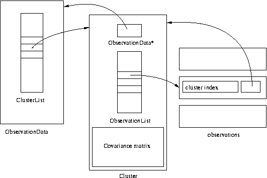
To enable adjustment of possibly correlated observations (like angles
derived from observed directions or already adjusted coordinates from
a previous adjustment) Gama has come with the concept of
clusters. Cluster is an object with a common
variance-covariance matrix and a list of pointers to observation
objects (distances, directions, angles, etc.). Weights were removed
from observation objects and replaced with a pointer to the cluster to
which the observation belong. All clusters are joined in a common
object ObservationData; similarly to observations, each cluster
contains a pointer to its parent Observation Data object.
Orientation shifts were separated from coordinates and are
stored in the cluster containing the bunch of directions and thus
number of orientations is not limited to one for a point.
This organisation of observational information has proved to be
effective. Template classes ObservationData and Cluster
are used as base classes both in gama-local and gama-g3
template <typename Observation>
  class ObservationData
  {
  public:
    ClusterList<Observation>  CL;

    ObservationData();
    ObservationData(const ObservationData& cod);
    ~ObservationData();

    ObservationData& operator=(const ObservationData& cod);
    template <typename P> void for_each(const P& p) const;
  };

template <typename Observation>
  class Cluster
  {
  public:
    const ObservationData<Observation>*     observation_data;
    ObservationList<Observation>            observation_list;
    typename Observation::CovarianceMatrix  covariance_matrix;

    Cluster(const ObservationData<Observation>* od);
    virtual ~Cluster();

    virtual Cluster* clone(const ObservationData<Observation>*) const = 0;
    double stdDev(int i) const;
    int size() const;
    void update();
    int  activeCount() const;
    typename Observation::CovarianceMatrix activeCov() const;
  };
The following template class PointBase for handling point
information is used in gama-g3. The template class
PointBase relies internally on std::map container but
comes with its own interface (in gama-local std::map
was used directly for storing points).
template <typename Point>
  class PointBase
  {
    typedef std::map<typename Point::Name, Point*>  Points;

  public:
    PointBase();
    PointBase(const PointBase& cod);
    ~PointBase();

    PointBase& operator=(const PointBase& cod);
    void put(const Point&);
    void put(Point*);
    Point*       find(const typename Point::Name&);
    const Point* find(const typename Point::Name&) const;
    void erase(const typename Point::Name&);
    void erase();

    class const_iterator;
    const_iterator  begin();
    const_iterator  end  ();

    class iterator;
    iterator  begin();
    iterator  end  ();
  };
Template classes ObservationData and PointBase are
defined in namespace GNU_gama and are located in the source
directory gnu_gama.
| [ < ] | [ > ] | [ << ] | [ Up ] | [ >> ] | [Top] | [Contents] | [Index] | [ ? ] |
| id | a | b, 1/f, f | description | |
| airy | 6377563.396 | 6356256.910 | Airy ellipsoid 1830 | [4] |
| airy_mod | 6377340.189 | 6356034.446 | Modified Airy | [4] |
| apl1965 | 6378137 | 298.25 | Appl. Physics. 1965 | [4] |
| andrae1876 | 6377104.43 | 300.0 | Andrae 1876 (Denmark, Iceland) | [4] |
| australian | 6378160 | 298.25 | Australian National 1965 | [3] |
| bessel | 6377397.15508 | 6356078.96290 | Bessel ellipsoid 1841 | [1] |
| bessel_nam | 6377483.865 | 299.1528128 | Bessel 1841 (Namibia) | [4] |
| clarke1858a | 6378361 | 6356685 | Clarke ellipsoid 1858 1st | [3] |
| clarke1858b | 6378558 | 6355810 | Clarke ellipsoid 1858 2nd | [3] |
| clarke1866 | 6378206.4 | 6356583.8 | Clarke ellipsoid 1866 | [3] |
| clarke1880 | 6378316 | 6356582 | Clarke ellipsoid 1880 | [3] |
| clarke1880m | 6378249.145 | 293.4663 | Clarke ellipsoid 1880 (modified) | [4] |
| cpm1799 | 6375738.7 | 334.29 | Comm. des Poids et Mesures 1799 | [4] |
| delambre | 6376428 | 311.5 | Delambre 1810 (Belgium) | [4] |
| engelis | 6378136.05 | 298.2566 | Engelis 1985 | [4] |
| everest1830 | 6377276.345 | 300.8017 | Everest 1830 | [4] |
| everest1848 | 6377304.063 | 300.8017 | Everest 1948 | [4] |
| everest1856 | 6377301.243 | 300.8017 | Everest 1956 | [4] |
| everest1869 | 6377295.664 | 300.8017 | Everest 1969 | [4] |
| everest_ss | 6377298.556 | 300.8017 | Everest (Sabah and Sarawak) | [4] |
| fisher1960 | 6378166 | 298.3 | Fisher 1960 (Mercury Datum) | [3] [4] |
| fisher1960m | 6378155 | 298.3 | Modified Fisher 1960 | [3] [4] |
| fischer1968 | 6378150 | 298.3 | Fischer 1968 | [4] |
| grs67 | 6378160 | 298.2471674270 | GRS 67 (IUGG 1967) | [4] |
| grs80 | 6378137 | 298.257222101 | Geodetic Reference System 1980 | [1] |
| hayford | 6378388 | 297 | Hayford 1909 (International) | [1] [3] |
| helmert | 6378200 | 298.3 | Helmert ellipsoid 1906 | [3] |
| hough | 6378270 | 297 | Hough | [4] |
| iau76 | 6378140 | 298.257 | IAU 1976 | [4] |
| international | 6378388 | 297 | International 1924 (Hayford 1909) | [1] [3] |
| kaula | 6378163 | 298.24 | Kaula 1961 | [4] |
| krassovski | 6378245 | 298.3 | Krassovski ellipsoid 1940 | [1] |
| lerch | 6378139 | 298.257 | Lerch 1979 | [4] |
| mprts | 6397300 | 191.0 | Maupertius 1738 | [4] |
| mercury | 6378166 | 298.3 | Mercury spheroid 1960 | [3] |
| merit | 6378137 | 298.257 | MERIT 1983 | [4] |
| new_intl | 6378157.5 | 6356772.2 | New International 1967 | [4] |
| nwl1965 | 6378145 | 298.25 | Naval Weapons Lab., 1965 | [4] |
| plessis | 6376523 | 6355863 | Plessis 1817 (France) | [4] |
| se_asia | 6378155 | 6356773.3205 | Southeast Asia | [4] |
| sgs85 | 6378136 | 298.257 | Soviet Geodetic System 85 | [4] |
| schott | 6378157 | 304.5 | Schott 1900 spheroid | [3] |
| sa1969 | 6378160 | 298.25 | South American Spheroid 1969 | [3] |
| walbeck | 6376896 | 6355834.8467 | Walbeck | [4] |
| wgs60 | 6378165 | 298.3 | WGS 60 | [4] |
| wgs66 | 6378145 | 298.25 | WGS 66 | [4] |
| wgs72 | 6378135 | 298.26 | WGS 72 | [4] |
| wgs84 | 6378137 | 298.257223563 | World Geodetic System 1984 | [1] |
| [1] | Milos Cimbalnik - Leos Mervart: Vyssi geodezie 1, 1997, Vydavatelstvi CVUT, Praha |
| [2] | Milos Cimbalnik: Derived Geometrical Constants of the Geodetic Reference System 1980, Studia geoph. et geod. 35 (1991), pp. 133-144, NCSAV, Praha |
| [3] | Glossary of the Mapping Sciences, Prepared by a Joint Committe of the American Society of Civil Engineers, American Congress on Surveying and Mapping and American Society for Photogrammetry and Remote Sensing (1994), USA, ISBN 1-57083-011-8, ISBN 0-7844-0050-4 |
| [4] | Gerald Evenden: proj - forward cartographic projection filter (rel. 4.3.3), http://www.remotesensing.org/proj |
| [ < ] | [ > ] | [ << ] | [ Up ] | [ >> ] | [Top] | [Contents] | [Index] | [ ? ] |
Spatial coordinates (X, Y, Z) can be easily computed from geographical ellipsoidal coordinates (B, L, H), where B is geographical latitude, L geographical longitude and H is elliposidal height, as
X = (N + H) cos B cos L Y = (N + H) cos B sin L Z = (N(1-e^2) + H)sin B |
where N = a/sqrt(1 - e^2 sin^2 B) is the radius of curvature in the prime vertical, e^2 = (a^2 - b^2)/a^2 is the first eccentricity for the given rotational ellipsoid (spheroid) with semi-major axis a and semi-minor axis b.
In the case of coordiante transformation from (X, Y, Z) to (B, L, H), the longitude is given by the formula
tan L = Y / X. |
Now we can introduce
D = sqrt(X^2 + Y^2), |
so that the cartesian system become (D, Z). Coordinates B and H are then usually computed by iteration with some starting value of B_0, for example
tan B_0 = Z/D/(1 - e^2), |
tan B = Z/D + N/(N+H) e^2 tan B, H = D / cos B = Z / sin B - N(1-e^2) |
B. R. Bowring described a closed formula(3) that is more effective and sufficiantly accurate and that is used in GNU Gama.
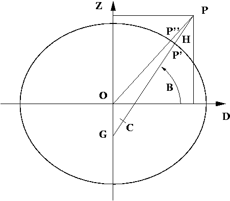
The centre of curvature C of the spheroid corresponding to P’ is the point
(e^2 a cos^3 u, -e’^2 b sin^3 u)),
where e’^2 = (a^2 - b^2)/b^2 is second eccentricity and u is the parametric latitude of the point P’, (1-e^2)N sin B = b sin u. Therefore
tan B = (Z + e’^2 b sin^3 u) / (D - e^2 a cos^3 u).
This is clearly an iterative solution; but it has been found that this formula is extremely accurate using the single first approximation for u for the tan u = (Z/D)(a/b). Maximum error in earth bound region is 3e-8 of sexagesimal arc seconds (5e-7 millimetres); maximum is 0.0018” (0.1 millimetres) at height H = 2a.
| [ < ] | [ > ] | [ << ] | [ Up ] | [ >> ] | [Top] | [Contents] | [Index] | [ ? ] |
g3::Modelg3::model documentation shall come here ...
namespace GNU_gama {  namespace g3 {


  class Model {
  public:

    typedef GNU_gama::PointBase<g3::Point>              PointBase;
    typedef GNU_gama::ObservationData<g3::Observation>  ObservationData;

    PointBase           *points;
    ObservationData     *obs;

    GNU_gama::Ellipsoid  ellipsoid;


    Model();
    ~Model();

    Point* get_point(const Point::Name&);
    void   write_xml(std::ostream& out) const;
    void   pre_linearization();
}}
| [ < ] | [ > ] | [ << ] | [ Up ] | [ >> ] | [Top] | [Contents] | [Index] | [ ? ] |
With gama-local come several companion command line tools, most
of them being conversion programs for various data formats.
| 7.1 gama-local-deformation | ||
| 7.2 gama-local-gkf2yaml | ||
| 7.3 gama-local-yaml2gkf | ||
| 7.4 gama-local-xml2sql | ||
| 7.5 gama-local-xml2txt | ||
| 7.6 krumm2gama-local |
| [ < ] | [ > ] | [ << ] | [ Up ] | [ >> ] | [Top] | [Contents] | [Index] | [ ? ] |
Program gama-local-deformation reads XML adjustment results files from
two dates (epochs), compute differences for adjusted points common in
both epochs, calculate the covariance matrix of the differences and
optionally renders the deformation diagram in SVG output file.
Usage: gama-local-deformation epoch1.xml epoch2.xml [--text file] [--svg file]
       gama-local-deformation --version
       gama-local-deformation --help

Options:

epoch1 and epoch2 are adjustment results in XML format of the surveying network.
           The program computes the shift vectors of common adjusted points
           and their corresponding covariance matrix.

--text     deformation analyses in textual format. If missing, standard
           output device is used (i.e. screen).
--svg      if defined, the program writes SVG image of the second epoch
           adjustment with standard deviation ellipses and points' shits.
           The network schema is available only in 2D (xy coordinates only).
--version
--help

Report bugs to: <bug-gama@gnu.org>
GNU gama home page: <https://www.gnu.org/software/gama/>
General help using GNU software: <https://www.gnu.org/gethelp/>
|

| [ < ] | [ > ] | [ << ] | [ Up ] | [ >> ] | [Top] | [Contents] | [Index] | [ ? ] |
Program gama-local-gkf2yaml converts input XML format of
gama-local (in Gama project usually denoted with
extension gkf) to yaml format.
gama-local-gkf2yaml input.gkf [output.yaml] |
| [ < ] | [ > ] | [ << ] | [ Up ] | [ >> ] | [Top] | [Contents] | [Index] | [ ? ] |
Program gama-local-yaml2gkf converts YAML input to XML imput format.
gama-local-yaml2gkf input.yaml [ output.gkf ] |
| [ < ] | [ > ] | [ << ] | [ Up ] | [ >> ] | [Top] | [Contents] | [Index] | [ ? ] |
Program gama-local-xml2sql converts gama-local XML input format (aka gkf) to SQL script.
Usage: gama-local-xml2sql configuration (xml_input|-) [sql_output|-] Convert XML adjustment input of gama-local to SQL |
| [ < ] | [ > ] | [ << ] | [ Up ] | [ >> ] | [Top] | [Contents] | [Index] | [ ? ] |
Conversion from adjustment XML output to text format.
Usage: gama-local-xml2txt [options] < std_input > std_output Convert XML adjustment output of gama-local to text format Options: --angles 400 | 360 --language en | ca | cz | du | fi | fr | hu | ru | ua --encoding utf-8 | iso-8859-2 | iso-8859-2-flat | cp-1250 | cp-1251 --help |
| [ < ] | [ > ] | [ << ] | [ Up ] | [ >> ] | [Top] | [Contents] | [Index] | [ ? ] |
GNU Gama sources come with an extensive set of testing data examples
in the directory tests where subdirectory tests/krumm
contains examples from the book by Friedhelm Krumm, Geodetic Network
Adjustment Examples, Geodätisches Institut Universität Stuttgart,
https://www.gis.uni-stuttgart.de, Rev. 3.5 January 20, 2020. All these
examples are distributed with GNU Gama with permission from the author.
Conversion program krumm2gama-local converts the examples data
format defined in the book to the gama-local XML input
format. For more details read the file
tests/krumm/input.README.md.
Conversion from data format used in Geodetic Network Adjustment Examples
by Friedhelm Krumm to XML input format of gama-local (GNU Gama)
https://www.gis.uni-stuttgart.de/lehre/campus-docs/adjustment_examples.pdf

     krumm2gama-local  input_file  [ output_file  ]
     krumm2gama-local < std_input  [ > std_output ]

Options:
-h, --help      this text
-v, --version   print program version
-e, --examples  add the following comment to the generated XML file

     This example is based on published material Geodetic Network Adjustment
     Examples by Friedhelm Krumm, Geodätisches Institut Universität Stuttgart,
     Rev. 3.5, January 20, 2020
|
| [ < ] | [ > ] | [ << ] | [ Up ] | [ >> ] | [Top] | [Contents] | [Index] | [ ? ] |
GNU Gama comes with a set of tests that provides gama-local test suite.
To run the test suite, go to the top-level Gama directory and type
$ make check |
You should see the names of the test suite files as they are processed, any other output indicates some problem. The output might be for example this
Entering directory 'gama/tests/gama-local' PASS: gama-local-version.sh PASS: gama-local-adjustment.sh PASS: gama-local-algorithms.sh PASS: gama-local-xml-xml.sh PASS: gama-local-html.sh PASS: gama-local-equivalents.sh PASS: gama-local-xml-results.sh PASS: gama-local-parameters.sh PASS: gama-local-export.sh PASS: gama-local-sqlite-reader.sh PASS: xmllint-gama-local-xsd.sh PASS: xmllint-gama-local-adjustment-xsd.sh ======================================================================== Testsuite summary for gama 2.29 ======================================================================== # TOTAL: 12 # PASS: 12 # SKIP: 0 # XFAIL: 0 # FAIL: 0 # XPASS: 0 # ERROR: 0 ======================================================================== |
Number of tests vary according to the configuration of your system. Tests that are always present are
gama-local-version gama-local-adjustment gama-local-algorithms gama-local-xml-xml gama-local-html gama-local-equivalents gama-local-xml-results gama-local-parameters gama-local-export |
Optional tests are
gama-local-sqlite-reader xmllint-gama-local-xsd xmllint-gama-local-adjustment-xsd |
which are included only if sqlite3 database support libraries and/or
xmllint program are installed.
You can also request more extra test configuring the project as
./configure --enable-extra-tests |
but be prepared that these extra test might take some time to finish.
| 8.1 Internal organisation |
| [ < ] | [ > ] | [ << ] | [ Up ] | [ >> ] | [Top] | [Contents] | [Index] | [ ? ] |
Gama-local tests are implemented as shell scripts that are stored in
gama/tests/gama-local directory. The scripts are generated from
corresponding .in files which are stored in
gama/tests/gama-local/script directory where are also stored
helper C++ programs called by the testing suite scripts. Generating
scripts and the build of helper programs is controlled from
gama/tests/gama-local/Makefile.am, where a list of testing data
files is also defined.
In gama/tests/gama-local directory are also stored detail
.log files for all tests together with corresponging
.trs (as in Test ReSults) files.
All files generated by the test suite are stored in
gama/tests/gama-local/script/2.29 (thus generated
files from different versions are not overwritten).
To run selected test individually, go to the directory
gama/tests/gama-local and start the test manually
$ cd gama/tests/gama-local $ ./test-name |
| [ < ] | [ > ] | [ << ] | [ Up ] | [ >> ] | [Top] | [Contents] | [Index] | [ ? ] |
| A.1 GNU Free Documentation License | License for copying this manual. |
| [ < ] | [ > ] | [ << ] | [ Up ] | [ >> ] | [Top] | [Contents] | [Index] | [ ? ] |
Version 1.1, March 2000
Copyright © 2000 Free Software Foundation, Inc. 51 Franklin Street, Fifth Floor, Boston, MA 02110-1301, USA Everyone is permitted to copy and distribute verbatim copies of this license document, but changing it is not allowed. |
The purpose of this License is to make a manual, textbook, or other written document free in the sense of freedom: to assure everyone the effective freedom to copy and redistribute it, with or without modifying it, either commercially or noncommercially. Secondarily, this License preserves for the author and publisher a way to get credit for their work, while not being considered responsible for modifications made by others.
This License is a kind of “copyleft”, which means that derivative works of the document must themselves be free in the same sense. It complements the GNU General Public License, which is a copyleft license designed for free software.
We have designed this License in order to use it for manuals for free software, because free software needs free documentation: a free program should come with manuals providing the same freedoms that the software does. But this License is not limited to software manuals; it can be used for any textual work, regardless of subject matter or whether it is published as a printed book. We recommend this License principally for works whose purpose is instruction or reference.
This License applies to any manual or other work that contains a notice placed by the copyright holder saying it can be distributed under the terms of this License. The “Document”, below, refers to any such manual or work. Any member of the public is a licensee, and is addressed as “you”.
A “Modified Version” of the Document means any work containing the Document or a portion of it, either copied verbatim, or with modifications and/or translated into another language.
A “Secondary Section” is a named appendix or a front-matter section of the Document that deals exclusively with the relationship of the publishers or authors of the Document to the Document’s overall subject (or to related matters) and contains nothing that could fall directly within that overall subject. (For example, if the Document is in part a textbook of mathematics, a Secondary Section may not explain any mathematics.) The relationship could be a matter of historical connection with the subject or with related matters, or of legal, commercial, philosophical, ethical or political position regarding them.
The “Invariant Sections” are certain Secondary Sections whose titles are designated, as being those of Invariant Sections, in the notice that says that the Document is released under this License.
The “Cover Texts” are certain short passages of text that are listed, as Front-Cover Texts or Back-Cover Texts, in the notice that says that the Document is released under this License.
A “Transparent” copy of the Document means a machine-readable copy, represented in a format whose specification is available to the general public, whose contents can be viewed and edited directly and straightforwardly with generic text editors or (for images composed of pixels) generic paint programs or (for drawings) some widely available drawing editor, and that is suitable for input to text formatters or for automatic translation to a variety of formats suitable for input to text formatters. A copy made in an otherwise Transparent file format whose markup has been designed to thwart or discourage subsequent modification by readers is not Transparent. A copy that is not “Transparent” is called “Opaque”.
Examples of suitable formats for Transparent copies include plain ASCII without markup, Texinfo input format, LaTeX input format, SGML or XML using a publicly available DTD, and standard-conforming simple HTML designed for human modification. Opaque formats include PostScript, PDF, proprietary formats that can be read and edited only by proprietary word processors, SGML or XML for which the DTD and/or processing tools are not generally available, and the machine-generated HTML produced by some word processors for output purposes only.
The “Title Page” means, for a printed book, the title page itself, plus such following pages as are needed to hold, legibly, the material this License requires to appear in the title page. For works in formats which do not have any title page as such, “Title Page” means the text near the most prominent appearance of the work’s title, preceding the beginning of the body of the text.
You may copy and distribute the Document in any medium, either commercially or noncommercially, provided that this License, the copyright notices, and the license notice saying this License applies to the Document are reproduced in all copies, and that you add no other conditions whatsoever to those of this License. You may not use technical measures to obstruct or control the reading or further copying of the copies you make or distribute. However, you may accept compensation in exchange for copies. If you distribute a large enough number of copies you must also follow the conditions in section 3.
You may also lend copies, under the same conditions stated above, and you may publicly display copies.
If you publish printed copies of the Document numbering more than 100, and the Document’s license notice requires Cover Texts, you must enclose the copies in covers that carry, clearly and legibly, all these Cover Texts: Front-Cover Texts on the front cover, and Back-Cover Texts on the back cover. Both covers must also clearly and legibly identify you as the publisher of these copies. The front cover must present the full title with all words of the title equally prominent and visible. You may add other material on the covers in addition. Copying with changes limited to the covers, as long as they preserve the title of the Document and satisfy these conditions, can be treated as verbatim copying in other respects.
If the required texts for either cover are too voluminous to fit legibly, you should put the first ones listed (as many as fit reasonably) on the actual cover, and continue the rest onto adjacent pages.
If you publish or distribute Opaque copies of the Document numbering more than 100, you must either include a machine-readable Transparent copy along with each Opaque copy, or state in or with each Opaque copy a publicly-accessible computer-network location containing a complete Transparent copy of the Document, free of added material, which the general network-using public has access to download anonymously at no charge using public-standard network protocols. If you use the latter option, you must take reasonably prudent steps, when you begin distribution of Opaque copies in quantity, to ensure that this Transparent copy will remain thus accessible at the stated location until at least one year after the last time you distribute an Opaque copy (directly or through your agents or retailers) of that edition to the public.
It is requested, but not required, that you contact the authors of the Document well before redistributing any large number of copies, to give them a chance to provide you with an updated version of the Document.
You may copy and distribute a Modified Version of the Document under the conditions of sections 2 and 3 above, provided that you release the Modified Version under precisely this License, with the Modified Version filling the role of the Document, thus licensing distribution and modification of the Modified Version to whoever possesses a copy of it. In addition, you must do these things in the Modified Version:
If the Modified Version includes new front-matter sections or appendices that qualify as Secondary Sections and contain no material copied from the Document, you may at your option designate some or all of these sections as invariant. To do this, add their titles to the list of Invariant Sections in the Modified Version’s license notice. These titles must be distinct from any other section titles.
You may add a section entitled “Endorsements”, provided it contains nothing but endorsements of your Modified Version by various parties—for example, statements of peer review or that the text has been approved by an organization as the authoritative definition of a standard.
You may add a passage of up to five words as a Front-Cover Text, and a passage of up to 25 words as a Back-Cover Text, to the end of the list of Cover Texts in the Modified Version. Only one passage of Front-Cover Text and one of Back-Cover Text may be added by (or through arrangements made by) any one entity. If the Document already includes a cover text for the same cover, previously added by you or by arrangement made by the same entity you are acting on behalf of, you may not add another; but you may replace the old one, on explicit permission from the previous publisher that added the old one.
The author(s) and publisher(s) of the Document do not by this License give permission to use their names for publicity for or to assert or imply endorsement of any Modified Version.
You may combine the Document with other documents released under this License, under the terms defined in section 4 above for modified versions, provided that you include in the combination all of the Invariant Sections of all of the original documents, unmodified, and list them all as Invariant Sections of your combined work in its license notice.
The combined work need only contain one copy of this License, and multiple identical Invariant Sections may be replaced with a single copy. If there are multiple Invariant Sections with the same name but different contents, make the title of each such section unique by adding at the end of it, in parentheses, the name of the original author or publisher of that section if known, or else a unique number. Make the same adjustment to the section titles in the list of Invariant Sections in the license notice of the combined work.
In the combination, you must combine any sections entitled “History” in the various original documents, forming one section entitled “History”; likewise combine any sections entitled “Acknowledgments”, and any sections entitled “Dedications”. You must delete all sections entitled “Endorsements.”
You may make a collection consisting of the Document and other documents released under this License, and replace the individual copies of this License in the various documents with a single copy that is included in the collection, provided that you follow the rules of this License for verbatim copying of each of the documents in all other respects.
You may extract a single document from such a collection, and distribute it individually under this License, provided you insert a copy of this License into the extracted document, and follow this License in all other respects regarding verbatim copying of that document.
A compilation of the Document or its derivatives with other separate and independent documents or works, in or on a volume of a storage or distribution medium, does not as a whole count as a Modified Version of the Document, provided no compilation copyright is claimed for the compilation. Such a compilation is called an “aggregate”, and this License does not apply to the other self-contained works thus compiled with the Document, on account of their being thus compiled, if they are not themselves derivative works of the Document.
If the Cover Text requirement of section 3 is applicable to these copies of the Document, then if the Document is less than one quarter of the entire aggregate, the Document’s Cover Texts may be placed on covers that surround only the Document within the aggregate. Otherwise they must appear on covers around the whole aggregate.
Translation is considered a kind of modification, so you may distribute translations of the Document under the terms of section 4. Replacing Invariant Sections with translations requires special permission from their copyright holders, but you may include translations of some or all Invariant Sections in addition to the original versions of these Invariant Sections. You may include a translation of this License provided that you also include the original English version of this License. In case of a disagreement between the translation and the original English version of this License, the original English version will prevail.
You may not copy, modify, sublicense, or distribute the Document except as expressly provided for under this License. Any other attempt to copy, modify, sublicense or distribute the Document is void, and will automatically terminate your rights under this License. However, parties who have received copies, or rights, from you under this License will not have their licenses terminated so long as such parties remain in full compliance.
The Free Software Foundation may publish new, revised versions of the GNU Free Documentation License from time to time. Such new versions will be similar in spirit to the present version, but may differ in detail to address new problems or concerns. See http://www.gnu.org/copyleft/.
Each version of the License is given a distinguishing version number. If the Document specifies that a particular numbered version of this License “or any later version” applies to it, you have the option of following the terms and conditions either of that specified version or of any later version that has been published (not as a draft) by the Free Software Foundation. If the Document does not specify a version number of this License, you may choose any version ever published (not as a draft) by the Free Software Foundation.
| [ < ] | [ > ] | [ << ] | [ Up ] | [ >> ] | [Top] | [Contents] | [Index] | [ ? ] |
To use this License in a document you have written, include a copy of the License in the document and put the following copyright and license notices just after the title page:
Copyright (C) year your name. Permission is granted to copy, distribute and/or modify this document under the terms of the GNU Free Documentation License, Version 1.1 or any later version published by the Free Software Foundation; with the Invariant Sections being list their titles, with the Front-Cover Texts being list, and with the Back-Cover Texts being list. A copy of the license is included in the section entitled ``GNU Free Documentation License''. |
If you have no Invariant Sections, write “with no Invariant Sections” instead of saying which ones are invariant. If you have no Front-Cover Texts, write “no Front-Cover Texts” instead of “Front-Cover Texts being list”; likewise for Back-Cover Texts.
If your document contains nontrivial examples of program code, we recommend releasing these examples in parallel under your choice of free software license, such as the GNU General Public License, to permit their use in free software.
| [ < ] | [ > ] | [ << ] | [ Up ] | [ >> ] | [Top] | [Contents] | [Index] | [ ? ] |
| Jump to: | <
A C D E F G H I N O P R S T V W Z |
|---|
| Jump to: | <
A C D E F G H I N O P R S T V W Z |
|---|
| [Top] | [Contents] | [Index] | [ ? ] |
Wikipedia, http://en.wikipedia.org/wiki/Surveying
gama-local can solve the project equations (1)
directly using algorithms Gram-Schmidt orthogonalisation or
Singular Value Decomposition, which generally yield numerically
more stable solution.
B. R. Bowring: Transformation from spatial to geographical coordinates, Survey Review XXIII, 181, July 1976
| [Top] | [Contents] | [Index] | [ ? ] |
gama-local
<gama-local> and <network>externgama-local
gama-local
gama-local
| [Top] | [Contents] | [Index] | [ ? ] |
This document was generated on February 17, 2024 using texi2html 1.82.
The buttons in the navigation panels have the following meaning:
| Button | Name | Go to | From 1.2.3 go to |
|---|---|---|---|
| [ < ] | Back | Previous section in reading order | 1.2.2 |
| [ > ] | Forward | Next section in reading order | 1.2.4 |
| [ << ] | FastBack | Beginning of this chapter or previous chapter | 1 |
| [ Up ] | Up | Up section | 1.2 |
| [ >> ] | FastForward | Next chapter | 2 |
| [Top] | Top | Cover (top) of document | |
| [Contents] | Contents | Table of contents | |
| [Index] | Index | Index | |
| [ ? ] | About | About (help) |
where the Example assumes that the current position is at Subsubsection One-Two-Three of a document of the following structure:
This document was generated on February 17, 2024 using texi2html 1.82.